REVIEW 3 major objections 5 minor 93 references
A fast food-freezing temperature estimation framework using optimally located sensors
T0 review · 3 major / 5 minor · reviewed 2026-08-11 · deepseek-v4-flash
Pith's one-line read A physics-informed reduced-order inverse framework, trained on turbulent freezing simulations, reconstructs the internal temperature field of a freezing salmon slice from sparse external sensors with errors near 1 percent.
desk verdict Competent proof-of-concept for ROM-based state estimation in food freezing, worth refereeing despite the synthetic-validation ceiling on its practical claims. read the letter →
The pith
A machine-rendered reading of the paper's core claim, the machinery that carries it, and where it could break.
The reading
What carries the argument
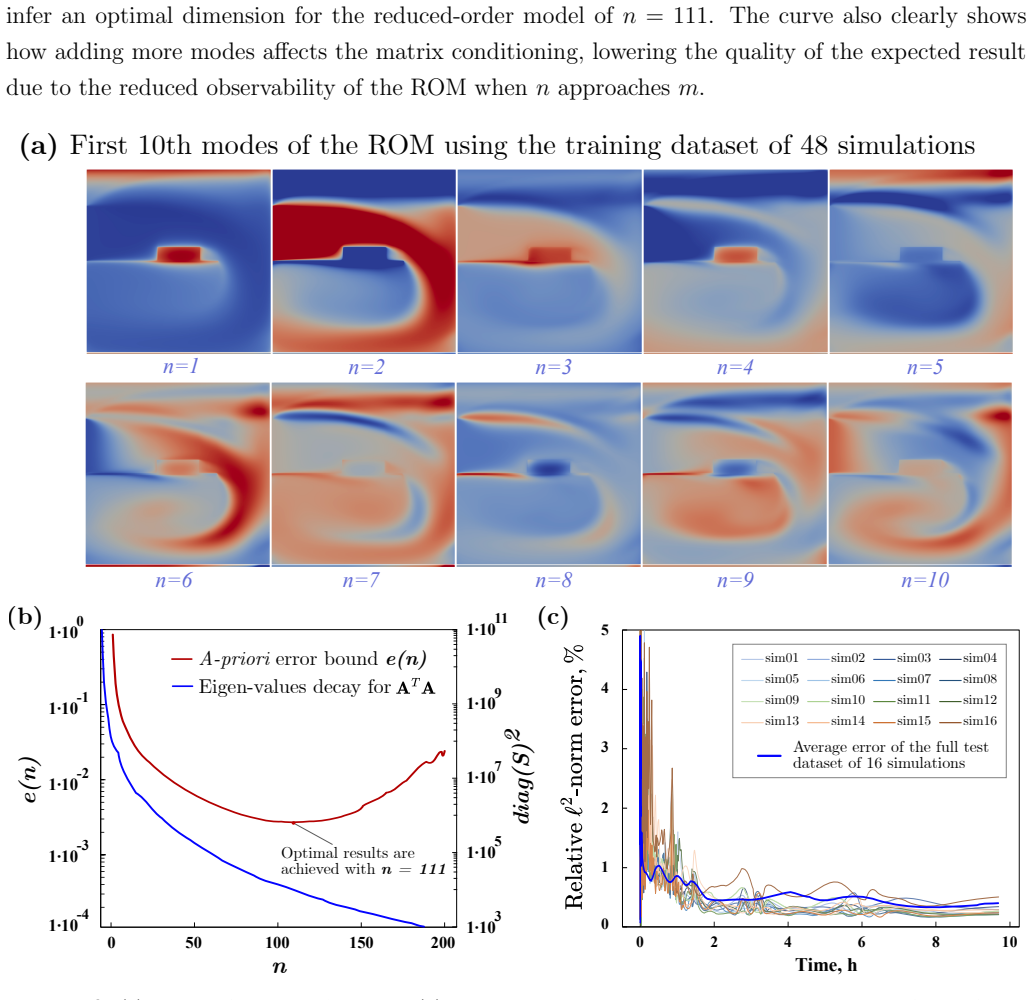
The central object is the reduced-order basis $\Phi$ — the first $n$ left singular vectors of a snapshot matrix built from 48 full-order turbulent freezing simulations — together with the cross-Gramian matrix $G = W^{\mathsf{T}}\Phi$ that couples it to the sensors. Each sensor is a column of the observation matrix $W$, a normalized indicator function (Riesz representer) over a measurement pixel, so measurements are local averages of the temperature field. The reconstruction solves the normal equations $G^{\mathsf{T}}G c = G^{\mathsf{T}}\ell$ in the $n$-dimensional space spanned by $\Phi$; well-posedness requires the number of measurements $m$ to exceed the ROM dimension $n$, and the error is controlled by the smallest singular value of $G$. The greedy algorithm places the next sensor to maximize that smallest singular value, equivalently to shrink the a priori bound $e(n) = \hat{S}_n^{-1} \, (\sum_{i>n} \sigma_i^2 / \sum_i \sigma_i^2)^{1/2}$, so the sensor layout is computed once, offline, without any dependence on the measurement values.
What would settle it
Place thermocouples at several depths inside a real salmon slice, run the freezer with the same boundary-condition range as the paper, mount the greedy-chosen sensors in the airflow, and compare the reconstructed internal temperature evolution against the thermocouple record; the framework is validated only if the reconstructed temperatures track the thermocouples to within the same few percent it achieves against its own simulation. A complementary check in simulation is to scramble the sensor positions from the greedy layout: if random layouts yield errors as low as the greedy one, the observability maximization is not carrying the accuracy claim.
Extended reading notes
Core claim
On the paper's own terms, the central claim is that a physics-informed reduced-order model — the first ~111 singular vectors of a 48-simulation snapshot set — together with a greedy sensor layout that maximizes the observability of that model, turns a severely underdetermined inverse problem into a well-posed one whose solution is the full temperature field. The quantified results are that the optimal 111-mode ROM reconstructs the temperature field over 16 held-out freezing simulations with peak errors near 5% at the start of freezing and errors below 1% for most of the process; that a greedy layout of 162 airflow sensors matches the accuracy of a regular 352-sensor array; and that restricting all sensors to the airflow, away from the food, still yields internal temperature errors of roughly 4 to 5%. The same reconstructed field supports derived quantities such as local freezing curves and freezing rates. The authors present the method as a proof of concept on synthetic data, with the full workflow — forward simulation, ROM training, sensor placement, and online reconstruction — designed to be transferable to experimental measurements.
Load-bearing premise
The load-bearing premise is that the forward URANS simulation — its k-omega SST turbulence closure, effective-heat-capacity phase change, and 2D geometry — faithfully represents the real freezing process at the operating Rayleigh numbers (Ra $> 10^{10}$); every reported reconstruction error is measured against that simulation's output, so any physical mismatch becomes reconstruction error.
Editorial extensions
If this is right
- Real-time monitoring becomes feasible: once the offline basis and sensor layout are built, each temperature reconstruction is just the solution of an $n \times n$ linear system with $n \approx 111$, so new measurements can be assimilated essentially as they arrive.
- Non-invasive quality control: temperature inside the food can be estimated from sensors in the airflow only, which is what makes the method practical for industrial freezers where probing the product is undesirable.
- Sensor economy: a greedy layout of 162 sensors matches the reconstruction accuracy of a regular 352-sensor thermo-camera array, and sparser layouts with roughly 56 sensors still keep time-averaged errors comparable to full-domain measurements.
- Derived quantities follow from the reconstructed field: local freezing curves and freezing rates can be computed at any point in the food, with local temperature errors below about 2% at control points, so quality-relevant indicators become available without extra sensors.
- The sensor placement is reusable: because the greedy optimization depends only on the ROM and the candidate sensor pool, not on the measurement values, the same layout serves any future freezing run in the same geometry without repeating the optimization.
Reading between the lines
- Beyond the paper: the same observability criterion — maximize the smallest singular value of the sensor-to-ROM cross-Gramian — should transfer to other conjugate heat-transfer monitoring tasks (thawing, baking, pasteurization, cryopreservation) where a snapshot dataset and a candidate sensor pool exist, so a natural extension is to test the pipeline on a different food geometry or a different phas
- Beyond the paper: because the reported ~1% error is measured against the URANS ground truth, the practical accuracy of the method in a real freezer hinges on the forward model's fidelity; an immediate testable extension is to repeat the reconstruction with experimental thermocouple data inside the salmon and report the error against those sensors instead of against the simulation.
- Beyond the paper: the error bound (14) suggests an adaptive experimental-design loop — add sensors only where the smallest singular value of $G$ would grow most — which the paper does not explore; this could yield layouts that respond to changing flow regimes or food loads.
Editorial analysis
A structured set of objections, weighed in public.
Referee Report
Summary. This paper presents a computational framework for estimating the full temperature field of a freezing salmon slab in a ventilated freezer from a limited number of temperature measurements. The forward model couples URANS airflow with a k-omega SST turbulence model, Boussinesq buoyancy, and an effective-heat-capacity phase-change model, solved by a WENO3 finite-volume scheme. A reduced basis is constructed by truncated SVD of snapshots from 48 training simulations sampled over a five-dimensional parameter range, and the inverse step is a ROM-regularized least-squares projection of the measurements onto that basis. Sensor positions are selected by a greedy algorithm that aims to maximize the smallest singular value of the cross-Gramian W^T Phi. Numerical experiments cover full-domain thermocamera-like measurements, measurements restricted to the airflow region outside the food, and comparisons of greedy versus regularly spaced sensor layouts, together with a benchmark using experimental thermocouple data.
Significance. If the claimed performance held at the operational conditions, the framework would be a practically useful tool for non-invasive, real-time monitoring of food freezing. The paper has several genuine strengths: the offline/online cost split is clearly quantified in Table 3, the sensor-placement criterion is based on an a-priori bound rather than on the measured values themselves, and the authors are explicit that the main validation is a proof-of-concept based on synthetic measurements. The methodological core (POD basis plus least-squares reconstruction) is standard, and the numerical behavior is internally consistent. However, the title-level claim of optimally located sensors and the abstract's claim of extrapolation under realistic turbulent flow conditions rest on validation that is almost entirely self-consistency with the training solver; this restricts the confidence that can be placed in the physical accuracy of the estimated fields.
major comments (3)
- [Section 4.3, Eq. (13)] The derivation of the a-priori bound contains a notation error that makes the displayed algebra invalid. After writing the singular value decomposition G = U_hat S_hat V_hat^T, the denominator is printed as d^T V^T Phi^T Phi V d, using the V from the snapshot SVD instead of V_hat; as written, the replacement of this denominator by d^T d is not justified. If V_hat was intended, the equality follows only after using both the orthonormality of the columns of Phi and the orthogonality of V_hat. Please correct this step or, more directly, invoke the standard fact that, for orthonormal Phi, inf_c ||G c|| / ||Phi c|| equals the smallest singular value of G. This is load-bearing because e(n) in Eq. (14) and the greedy criterion in Algorithm 1 are both derived from this bound.
- [Sections 2.4, 3.2, 5.1, 5.3] The operating regime is defined by Ra > 10^10, and the abstract claims efficient extrapolation from external measurements under realistic turbulent flow conditions. However, the forward solver is validated in Section 3.2 at Ra = 6.81e7 (P1) and Ra = 1.58e9 (P2), and all reconstruction errors in Sections 5.1, 5.3, and 5.4 are computed against the output of the same FVM solver that generated the training snapshots. The only experimental comparison, Section 5.2, uses a single-parameter ROM built from one low-Rayleigh simulation and does not exercise the external-only, high-Rayleigh setting that is the central claim. The reported ~1% errors therefore bound the ROM and inverse error conditional on the forward model being exact, not the error against real freezing behavior at Ra > 10^10. The claims should be reframed accordingly, or the paper should include a high-Rayleigh experimental or independent benchmark.
- [Section 4.3, Remark] The statement that the greedy selection guarantees beta(m*) >= beta(m_sub) for any other selection of m measurements is stronger than what a stepwise greedy procedure can establish. Greedy algorithms of this type are locally optimal at each addition but are not globally optimal over all m-sensor sets in general. This overstatement matters because optimally located sensors is a central claim of the paper; please either prove the global property for this particular objective or soften the remark to describe the bound in Eq. (14) as an observability criterion that is tested numerically.
minor comments (5)
- [Keywords] The keyword list contains the typo 'Inverse Problemas' and should read 'Inverse Problems'.
- [Figure 8] The figure states 'Sensor size (Voxel) = 0.2 x 0.2 cm', while the text of Section 5.1 says pixels of size 2 x 2 cm^2; the units and numbers should be made consistent.
- [Section 3.3] The reported mesh parameters appear inconsistent: hmin,2 = 7.2e-3 is larger than hmax,2 = 1.8e-3, which would make the stated minimum larger than the stated maximum for the second mesh.
- [Section 4.3, Eq. (14)] The word 'enumerator' should be 'numerator' in the sentence discussing the bound.
- [Sections 5.4 and Figures 15-16] The text alternates between m = 52 and m1 = 56 for the smallest sensor set; the notation should be unified, and the caption 'Greedy A.(m2 = 162)' appears incomplete.
Circularity Check
Minor self-citation in the ground-truth assumption; the ROM/inverse derivation itself is self-contained and not circular.
-
other
[Section 2, paragraph 3 (2D setup and ground-truth assumption)]
"We also performed a validation with experimental data previously published, which confirms that the use of the 2D model is adequate for the physical situation studied [65]. In that article, the importance of using ad-hoc turbulence models to describe the freezing evolution was discussed in detail, with URANS strategies being sufficiently accurate and efficient to reproduce experimental results. Since the key novelty of this article is the inverse estimation, we accept the 2D direct solution and use the 2D results as the ground truth values."
The evaluation protocol treats the forward solver's output as the ground truth T_GT for all reconstruction tests. The claim that this forward model is adequate at the stated operating regime (Ra>10^10) leans on [65], a prior article by co-author Rivera, whereas the in-paper benchmarks (P1, P2) are at Ra=6.81e7 and 1.58e9. This is a self-citation used to justify the input model. It is not a derivation step: the ROM construction, PBDW least-squares inversion, and greedy sensor placement are fully specified in Sections 4 and 5 and do not reduce to [65]. Thus it is a minor supporting self-citation rather than a load-bearing circular argument.
full rationale
The derivation chain is self-contained. The forward FVM solver (Section 3) generates snapshots; the ROM is obtained by truncated SVD of those snapshots (Section 4.2); the reconstruction solves the normal equations G^T G c = G^T ell with G = W^T Phi (Eqs. 9-10); and the sensor placement is computed from Phi and the observation matrix W only, independent of measurement values (Algorithm 1). No fitted parameter is renamed as a prediction, and no uniqueness theorem or ansatz is imported from the authors' prior work. The use of the same forward solver for training data, test measurements, and ground truth is a validation limitation rather than a circular reduction: the ROM is not fitted to the test measurements, and the reported errors measure the ROM's interpolation quality within the model's solution manifold. The only mildly circular element is the self-citation [65] used to justify accepting the 2D URANS solution as ground truth at the target regime, while the paper's own benchmarks are at lower Rayleigh numbers. This does not infect the inverse-method derivation, so the appropriate score is 2.
Assumptions & free parameters
free parameters (2)
- ROM dimension n =
n=111 for the main test, n=86 for the experimental validation
- BDF blend coefficient χ =
0.52
assumptions (5)
- standard math A-priori error bound (12) for PBDW/ROM state estimation
- domain assumption The URANS k-omega SST model accurately describes the turbulent airflow in the target regime (Ra>10^10)
- domain assumption The 2D mid-plane model is representative of the freezing cabinet
- domain assumption The effective heat capacity method captures the phase change behavior
- domain assumption Sensor measurements are linear functionals of the temperature field
Cite this review
Pith. "Pith review of A fast food-freezing temperature estimation framework using optimally located sensors." pith.science (2026). https://pith.science/paper/7T6TBRQA
@misc{pith2026241219387,
  author       = {Pith},
  title        = {Pith review of: A fast food-freezing temperature estimation framework using optimally located sensors},
  year         = {2026},
  howpublished = {\url{https://pith.science/paper/7T6TBRQA}},
  note         = {Machine review of arXiv:2412.19387}
}
read the original abstract
This article presents and assesses a framework for estimating temperature fields in real time for food-freezing applications, significantly reducing computational load while ensuring accurate temperature monitoring, which represents a promising technological tool for optimizing and controlling food engineering processes. The strategy is based on (i) a mathematical model of a convection-dominated problem coupling thermal convection and turbulence, and (ii) a least-squares approach for solving the inverse data assimilation problem, regularized by projecting the governing dynamics onto a reduced-order model (ROM). The unsteady freezing process considers a salmon slice in a freezer cabinet, modeled with temperature-dependent thermophysical properties. The forward problem is approximated using a third-order WENO finite volume solver, including an optimized second-order backward scheme for time discretization. We employ our data assimilation framework to reconstruct the temperature field based on a limited number of sensors and to estimate temperature distributions within frozen food. Sensor placement is optimized using a novel greedy algorithm, which maximizes the observability of the reduced-order dynamics for a fixed set of sensors. The proposed approach allows efficient extrapolation from external sensor measurements to the internal temperature of the food under realistic turbulent flow conditions, which is crucial for maintaining food quality.
Figures


Figures from the paper (14 more)




Reference graph
Works this paper leans on
-
[1]
Food preservation techniques and nanotechnology for increased shelf life of fruits, vegetables, beverages and spices: a review,
A. Sridhar, M. Ponnuchamy, P. S. Kumar, and A. Kapoor, “Food preservation techniques and nanotechnology for increased shelf life of fruits, vegetables, beverages and spices: a review,” Environmental Chemistry Letters , vol. 19, pp. 1715–1735, 2021
2021
-
[2]
Novel synergistic freezing methods and technologies for enhanced food product quality: A critical review,
R. Hu, M. Zhang, W. Liu, A. S. Mujumdar, and B. Bai, “Novel synergistic freezing methods and technologies for enhanced food product quality: A critical review,” Comprehensive Reviews in Food Science and Food Safety , vol. 21, no. 2, pp. 1979–2001, 2022
1979
-
[3]
Conjugate turbulent natural heat convection and solid food freezing modelling: Effects of position and number of pieces of salmon on the cooling rate,
N. P. Gonz´ alez, D. R. Rivera, and N. O. Moraga, “Conjugate turbulent natural heat convection and solid food freezing modelling: Effects of position and number of pieces of salmon on the cooling rate,” Thermal Science and Engineering Progress , vol. 26, p. 101101, 2021
2021
-
[4]
Effect of freezing rate on the quality of frozen strawberries (fragaria x ananassa),
D. L. Da Silva, A. S. Silveira, A. F. Ronzoni, and C. J. Hermes, “Effect of freezing rate on the quality of frozen strawberries (fragaria x ananassa),” International Journal of Refrigeration, vol. 144, pp. 46–54, 2022
2022
-
[5]
The physics of freezing and melting in the presence of flows,
Y. Du, E. Calzavarini, and C. Sun, “The physics of freezing and melting in the presence of flows,” Nature Reviews Physics , vol. 6, no. 11, pp. 676–690, 2024
2024
-
[6]
Recent advances in multiscale CFD modelling of cooling processes and systems for the agrifood industry,
C. K. Ajani, Z. Zhu, and D.-W. Sun, “Recent advances in multiscale CFD modelling of cooling processes and systems for the agrifood industry,”Critical Reviews In Food Science and Nutrition, vol. 61, no. 15, pp. 2455–2470, 2021
2021
-
[7]
Application of computational fluid dynamics simulations in food industry,
A. Szpicer, W. Bi´ nkowska, I. Wojtasik-Kalinowska, S. Salih, and A. P´ o ltorak, “Application of computational fluid dynamics simulations in food industry,” European Food Research and Technology, vol. 249, no. 6, pp. 1411–1430, 2023
2023
-
[8]
Improvement and Development of Physical Field Drying Technology: Principles, Models, Optimizations and Hybrids,
N. Ouyang, H. Ma, D. Liu, L. Guo, Y. Guo, and Y. Wang, “Improvement and Development of Physical Field Drying Technology: Principles, Models, Optimizations and Hybrids,” Food Engineering Reviews, pp. 1–28, 2025
2025
Show all 93 references
-
[9]
Predicting local surface heat transfer coefficients by different turbulentk- ϵ models to simulate heat and moisture transfer during air-blast chilling,
Z. Hu and D.-W. Sun, “Predicting local surface heat transfer coefficients by different turbulentk- ϵ models to simulate heat and moisture transfer during air-blast chilling,” International Journal of Refrigeration, vol. 24, no. 7, pp. 702–717, 2001
2001
-
[10]
Advantages in predicting conjugate freezing of meat in a domestic freezer by CFD with turbulence κ-ϵ 3D model and a local exergy destruction analysis,
N. O. Moraga and D. R. Rivera, “Advantages in predicting conjugate freezing of meat in a domestic freezer by CFD with turbulence κ-ϵ 3D model and a local exergy destruction analysis,” International Journal of Refrigeration , vol. 126, pp. 76–87, 2021
2021
-
[11]
A. Ray, P. Minz, and C. Sinha, “Framework for accurate estimation of freezing time and convec- tive heat transfer coefficient for freezing of a food product in domestic refrigerator: a numerical and simulation modeling approach,” Multiscale and Multidisciplinary Modeling, Expe...
2024
-
[12]
Validated numerical model of heat transfer in the forced air freezing of bulk packed whole chickens,
D. K. Hoang, S. J. Lovatt, J. R. Olatunji, and J. K. Carson, “Validated numerical model of heat transfer in the forced air freezing of bulk packed whole chickens,” International Journal of Refrigeration, vol. 118, pp. 93–103, 2020. 31
2020
-
[13]
Experimentally validated cfd-tool for a freezing simulation in a small-scale freeze-dryer,
E. Piechnik, J. Smolka, M. Palacz, I. Tolstorebrov, T. Eikevik, M. Stebel, M. Haida, A. Nowak, A. Ciesielska, and J. Bodys, “Experimentally validated cfd-tool for a freezing simulation in a small-scale freeze-dryer,” Journal of Food Engineering, vol. 367, p. 111888, 2024
2024
-
[14]
Effect of fan speed, sample orien- tation, and tray structure on heat transfer and food freezing time in batch air blast freezer,
Z. Xu, M. Redo, Y. Llave, Y. Koga, and M. Watanabe, “Effect of fan speed, sample orien- tation, and tray structure on heat transfer and food freezing time in batch air blast freezer,” International Journal of Thermal Sciences , vol. 214, p. 109915, 2025
2025
-
[16]
One-dimensional finite- difference modeling on temperature history and freezing time of individual food,
Z. Wang, H. Wu, G. Zhao, X. Liao, F. Chen, J. Wu, and X. Hu, “One-dimensional finite- difference modeling on temperature history and freezing time of individual food,” Journal of Food Engineering, vol. 79, no. 2, pp. 502–510, 2007
2007
-
[17]
FDM for the freezing process of a slab using integral average properties,
S. Ferreira, “FDM for the freezing process of a slab using integral average properties,” Interna- tional Journal of Refrigeration , vol. 119, pp. 326–339, 2020
2020
-
[18]
Simulation of Transport Phenomena for Microwave Freeze-Drying of Potato Slices Using Finite Element Analysis,
N. Sujinda and J. Varith, “Simulation of Transport Phenomena for Microwave Freeze-Drying of Potato Slices Using Finite Element Analysis,” Food Frontiers, vol. 6, no. 1, pp. 532–548, 2025
2025
-
[19]
Computational heat transfer analysis of liquid food in a heat exchanger with vary- ing stirrer settings in a nonclassical continuum framework,
M. Khan, “Computational heat transfer analysis of liquid food in a heat exchanger with vary- ing stirrer settings in a nonclassical continuum framework,” Numerical Heat Transfer, Part B: Fundamentals, pp. 1–20, 2024
2024
-
[20]
Thermal Analysis of Conjugate Con- vective Flow in a Vented Chamber Featuring Different Heat-Generating Solid Objects,
M. Zaman, F. Ahmed, M. Shuvo, N. Deb, and S. Saha, “Thermal Analysis of Conjugate Con- vective Flow in a Vented Chamber Featuring Different Heat-Generating Solid Objects,”Arabian Journal for Science and Engineering , pp. 1–15, 2024
2024
-
[21]
Predicting heat conduction during solidification of a food inside a freezer due to natural convection,
N. O. Moraga and H. G. Barraza, “Predicting heat conduction during solidification of a food inside a freezer due to natural convection,” Journal of Food Engineering , vol. 56, no. 1, pp. 17–26, 2003
2003
-
[22]
Experimental and numerical characterization of food dehydration during freezing,
V. Mulot, H. Benkhelifa, D. Pathier, F.-T. Ndoye, and D. Flick, “Experimental and numerical characterization of food dehydration during freezing,” Journal of Food Engineering , vol. 263, pp. 13–24, 2019
2019
-
[23]
Freezing of foods: Mathematical and experimental aspects,
P. Takhar, “Freezing of foods: Mathematical and experimental aspects,” Food Engineering Reviews, vol. 9, 2017
2017
-
[24]
Concept of Com- putational Fluid Dynamics design and analysis tool for food industry: A bibliometric,
M. Muktiarni, N. I. Rahayu, A. Nurhayati, A. D. Bachari, and A. Ismail, “Concept of Com- putational Fluid Dynamics design and analysis tool for food industry: A bibliometric,” CFD Letters, vol. 16, no. 2, p. 1–23, 2023
2023
-
[25]
Exploring mathematical modeling and cfd in con- vective drying of fruits and vegetables: A review,
E. Arpaci, C. Atayılmaz, and Z. Gemici, “Exploring mathematical modeling and cfd in con- vective drying of fruits and vegetables: A review,” Food and Bioprocess Technology, pp. 1–28, 2024. 32
2024
-
[26]
Inverse problems in food engineering: A review,
R. S. Reddy, D. Arepally, and A. K. Datta, “Inverse problems in food engineering: A review,” Journal of Food Engineering, vol. 319, p. 110909, 2022
2022
-
[27]
Moisture diffusivity coefficient estimation in solid food by inversion of a numerical model,
A. Fabbri, C. Cevoli, and R. Troncoso, “Moisture diffusivity coefficient estimation in solid food by inversion of a numerical model,” Food Research International, vol. 56, pp. 63–67, 2014
2014
-
[28]
Estimation of the energy requirement of bread during baking by inverse heat transfer method,
S. R. Ravula, D. Arepally, and A. K. Datta, “Estimation of the energy requirement of bread during baking by inverse heat transfer method,” Journal of Thermal Analysis and Calorimetry , vol. 148, no. 23, pp. 13 297–13 311, 2023
2023
-
[29]
Inverse method for the simultaneous estimation of the thermophysical properties of foods at freezing temperatures,
I. Cornejo, G. Cornejo, C. Ram ´ ırez, S. Almonacid, and R. Simpson, “Inverse method for the simultaneous estimation of the thermophysical properties of foods at freezing temperatures,” Journal of Food Engineering, vol. 191, pp. 37–47, 2016
2016
-
[30]
Inverse estimation of thermal parameters and friction co- efficient during warm flat rolling process,
V. Yadav, A. Singh, and U. Dixit, “Inverse estimation of thermal parameters and friction co- efficient during warm flat rolling process,” International Journal of Mechanical Sciences , vol. 96-97, pp. 182–198, 2015
2015
-
[31]
Inverse estimation of the transient-state stress distribution in the power boiler pressure components,
P. Duda, “Inverse estimation of the transient-state stress distribution in the power boiler pressure components,” International Journal of Mechanical Sciences , vol. 107, pp. 201–214, 2016
2016
-
[32]
Coupled data assimilation and parameter estimation in coupled ocean- atmosphere models: A review,
S. Zhang, Z. Liu, X. Zhang, X. Wu, G. Han, Y. Zhao, X. Yu, C. Liu, Y. Liu, S. Wu, F. Lu, M. Li, and X. Deng, “Coupled data assimilation and parameter estimation in coupled ocean- atmosphere models: A review,” Climate Dynamics , vol. 54, no. 11-12, pp. 5127–5144, 2020
2020
-
[33]
Reduced basis homogenization of thermal and elastic properties for periodic composite materials,
Q. X. Pham and K. Lee, “Reduced basis homogenization of thermal and elastic properties for periodic composite materials,” International Journal of Mechanical Sciences , p. 109801, 2024
2024
-
[34]
A survey on deep learning tools dealing with data scarcity: definitions, challenges, solutions, tips, and applications,
L. Alzubaidi, J. Bai, A. Al-Sabaawi, J. Santamar ´ ıa, A. S. Albahri, B. S. N. Al-Dabbagh, M. A. Fadhel, M. Manoufali, J. Zhang, A. H. Al-Timemy et al. , “A survey on deep learning tools dealing with data scarcity: definitions, challenges, solutions, tips, and applications,” J...
2023
-
[35]
A real-time variational data assimilation method with data-driven model enrichment for time-dependent problems,
W. Haik, Y. Maday, and L. Chamoin, “A real-time variational data assimilation method with data-driven model enrichment for time-dependent problems,” Computer Methods in Applied Mechanics and Engineering , vol. 405, p. 115868, 2023
2023
-
[36]
Respecting causality for training physics-informed neural networks,
S. Wang, S. Sankaran, and P. Perdikaris, “Respecting causality for training physics-informed neural networks,” Computer Methods in Applied Mechanics and Engineering, vol. 421, p. 116813, 2024
2024
-
[37]
From PINNs to PIKANs: recent advances in physics-informed machine learning,
J. D. Toscano, V. Oommen, A. J. Varghese, Z. Zou, N. Ahmadi Daryakenari, C. Wu, and G. E. Karniadakis, “From PINNs to PIKANs: recent advances in physics-informed machine learning,” Machine Learning for Computational Science and Engineering , vol. 1, no. 1, p. 15, 2025
2025
-
[38]
Data-driven modeling of an oscillating surge wave energy converter using dynamic mode decomposition,
B. Lydon, B. Polagye, and S. Brunton, “Data-driven modeling of an oscillating surge wave energy converter using dynamic mode decomposition,” Journal of Renewable and Sustainable Energy, vol. 17, no. 2, p. 024703, 03 2025. 33
2025
-
[39]
Physics-informed neural networks for parameter estimation in blood flow models,
J. Garay, J. Dunstan, S. Uribe, and F. S. Costabal, “Physics-informed neural networks for parameter estimation in blood flow models,” Computers in Biology and Medicine , vol. 178, p. 108706, 2024
2024
-
[40]
Maximumly weighted iteration for solving inverse problems in dynamics,
X. Yu, C. Cheng, Y. Yang, M. Du, Q.He, and Z. Peng, “Maximumly weighted iteration for solving inverse problems in dynamics,” International Journal of Mechanical Sciences , vol. 247, p. 108169, 2023
2023
-
[41]
Accurate state of temperature esti- mation for lithium-ion batteries based on square root cubature Kalman filter,
J. Shen, Z.Zhang, S. Shen, Y. Zhang, Z. Chen, and Y. Liu, “Accurate state of temperature esti- mation for lithium-ion batteries based on square root cubature Kalman filter,” Applied Thermal Engineering, vol. 242, p. 122452, 2024
2024
-
[42]
Time periodic natural convection heat transfer in a nano-encapsulated phase-change suspension,
A. Hajjar, S. Mehryan, and M. Ghalambaz, “Time periodic natural convection heat transfer in a nano-encapsulated phase-change suspension,” International Journal of Mechanical Sciences , vol. 166, p. 105243, 2020
2020
-
[43]
A reduced basis method for parametrized variational inequalities applied to contact mechanics,
A. Benaceur, A. Ern, and V. Ehrlacher, “A reduced basis method for parametrized variational inequalities applied to contact mechanics,” International Journal for Numerical Methods in Engineering, vol. 121, no. 6, pp. 1170–1197, 2020
2020
-
[44]
Approximation of large-scale dynamical systems: An overview
C. Antoulas and C. Sorensen, “Approximation of large-scale dynamical systems: An overview.” International Journal of Applied Mathematics and Computer Science , 2001
2001
-
[45]
Randomized compression of rank-structured matrices accelerated with graph coloring,
J. L. and P.-G. M., “Randomized compression of rank-structured matrices accelerated with graph coloring,” Journal of Computational and Applied Mathematics , vol. 451, p. 116044, 2024
2024
-
[46]
Friedrichs’ systems discretized with the dgm: domain de- composable model order reduction and graph neural networks approximating vanishing viscosity solutions,
F. Romor, D. Torlo, and G. Rozza, “Friedrichs’ systems discretized with the dgm: domain de- composable model order reduction and graph neural networks approximating vanishing viscosity solutions,” Journal of Computational Physics , vol. 531, p. 113915, 2025
2025
-
[47]
Higher order dynamic mode decomposition to model reacting flows,
A. Corrochano, G. D’Alessio, A.Parente, and S. Le Clainche, “Higher order dynamic mode decomposition to model reacting flows,” International Journal of Mechanical Sciences , vol. 249, p. 108219, 2023
2023
-
[48]
Reduced-order modelling based on non-linear modes,
C. Mazzilli, P. Gon¸ calves, and G. Franzini, “Reduced-order modelling based on non-linear modes,” International Journal of Mechanical Sciences , vol. 214, p. 106915, 2022
2022
-
[49]
Frangos, Y
M. Frangos, Y. Marzouk, K. Willcox, and B. van Bloemen Waanders, Surrogate and Reduced- Order Modeling: A Comparison of Approaches for Large-Scale Statistical Inverse Problems . John Wiley & Sons, Ltd, 2010, ch. 7, pp. 123–149
2010
-
[50]
Benner, M
P. Benner, M. Ohlberger, A. Cohen, and K. Willcox, Model reduction and approximation: theory and algorithms . SIAM, 2017
2017
-
[51]
Adaptive pbdw approach to state estimation: Noisy observations; user-defined update spaces,
Y. Maday and T. Taddei, “Adaptive pbdw approach to state estimation: Noisy observations; user-defined update spaces,” SIAM Journal on Scientific Computing , vol. 41, no. 4, pp. B669– B693, 2019. 34
2019
-
[52]
A parameterized-background data-weak approach to variational data assimilation: formulation, analysis, and application to acoustics,
Y. Maday, A. T. Patera, J. D. Penn, and M. Yano, “A parameterized-background data-weak approach to variational data assimilation: formulation, analysis, and application to acoustics,” International Journal for Numerical Methods in Engineering , vol. 102, no. 5, pp. 933–965, 2015
2015
-
[53]
Optimal reduced model algorithms for data-based state estimation,
A. Cohen, W. Dahmen, R. DeVore, J. Fadili, O. Mula, and J. Nichols, “Optimal reduced model algorithms for data-based state estimation,” SIAM Journal on Numerical Analysis , vol. 58, no. 6, pp. 3355–3381, 2020
2020
-
[54]
Fast reconstruction of 3D blood flows from Doppler ultrasound images and reduced models,
F. Galarce, J. Gerbeau, D. Lombardi, and O. Mula, “Fast reconstruction of 3D blood flows from Doppler ultrasound images and reduced models,” Computer Methods in Applied Mechanics and Engineering, vol. 375, p. 113559, 2021
2021
-
[55]
Reconstructing haemodynamics quantities of interest from Doppler ultrasound imaging,
F. Galarce, D. Lombardi, and O. Mula, “Reconstructing haemodynamics quantities of interest from Doppler ultrasound imaging,” International Journal for Numerical Methods in Biomedical Engineering, 2021
2021
-
[56]
Displacement and pressure reconstruction from magnetic resonance elastography images: Application to an In Silico brain model,
F. Galarce, K. Tabelow, J. Polzehl, C. Papanikas, V. Vavourakis, L. Lilaj, I. Sack, and A. Ca- iazzo, “Displacement and pressure reconstruction from magnetic resonance elastography images: Application to an In Silico brain model,” SIAM Journal on Imaging Sciences , vol. 16, no...
2023
-
[57]
Bias and multiscale correction methods for variational state estimation,
F. Galarce, J. Mura, and A. Caiazzo, “Bias and multiscale correction methods for variational state estimation,” Applied Mathematical Modelling , vol. 138, p. 115761, 2025
2025
-
[58]
Greedy selection of optimal location of sensors for uncertainty reduction in seismic moment tensor inversion,
B. M. Dia, M. Fehler, S. I. Kaka, A. Scarinci, U. bin Waheed, and C. Gu, “Greedy selection of optimal location of sensors for uncertainty reduction in seismic moment tensor inversion,” Journal of Computational Physics , vol. 519, 2024
2024
-
[59]
Sensor placement by maximal projection on minimum eigenspace for linear inverse problems,
C. Jiang, Y. C. Soh, and H. Li, “Sensor placement by maximal projection on minimum eigenspace for linear inverse problems,” IEEE Transactions on Signal Processing, vol. 64, no. 21, pp. 5595– 5610, 2016
2016
-
[60]
Group greedy method for sensor placement,
C. Jiang, Z. Chen, R. Su, and Y. C. Soh, “Group greedy method for sensor placement,” IEEE Transactions on Signal Processing, vol. 67, no. 9, pp. 2249–2262, 2019
2019
-
[61]
Data-driven sparse sensor place- ment for reconstruction: Demonstrating the benefits of exploiting known patterns,
K. Manohar, B. W. Brunton, J. N. Kutz, and S. L. Brunton, “Data-driven sparse sensor place- ment for reconstruction: Demonstrating the benefits of exploiting known patterns,” IEEE Con- trol Systems Magazine , vol. 38, no. 3, pp. 63–86, 2018
2018
-
[62]
Greedy algorithms for optimal measurements selection in state estimation using reduced models,
P. Binev, A. Cohen, O. Mula, and J. Nichols, “Greedy algorithms for optimal measurements selection in state estimation using reduced models,” SIAM/ASA Journal on Uncertainty Quan- tification, vol. 6, no. 3, pp. 1101–1126, 2018
2018
-
[63]
Dynamical approximation and sensor placement for filtering problems,
O. Mula, C. Pagliantini, and F. Vismara, “Dynamical approximation and sensor placement for filtering problems,” SIAM Journal on Scientific Computing , vol. 47, no. 1, pp. A403–A429, 2025
2025
-
[64]
Sparse wasserstein barycenters and application to reduced order modeling,
M. Do, J. Feydi, and O. Mula, “Sparse wasserstein barycenters and application to reduced order modeling,” Journal of Scientific Computing , vol. 102, 2025. 35
2025
-
[65]
Energy analysis of convective freezer cabinet with PCMs and salmon-fillet during charging, discharging and normal operation processes by CFD modeling,
D. R. Rivera and N. O. Moraga, “Energy analysis of convective freezer cabinet with PCMs and salmon-fillet during charging, discharging and normal operation processes by CFD modeling,” Journal of Energy Storage , vol. 83, p. 110558, 2024
2024
-
[66]
Control of ice crystal nucleation and growth during the food freezing process,
G. Jia, Y. Chen, A. Sun, and V. Orlien, “Control of ice crystal nucleation and growth during the food freezing process,” Comprehensive Reviews in Food Science and Food Safety , vol. 21, no. 3, pp. 2433–2454, 2022
2022
-
[67]
Regulating ice formation for enhancing frozen food quality: Materials, mechanisms and challenges,
L. Sun, Z. Zhu, and D. Sun, “Regulating ice formation for enhancing frozen food quality: Materials, mechanisms and challenges,” Trends in Food Science & Technology , vol. 139, p. 104116, 2023
2023
-
[68]
Effects of relative humidity on dry-aged beef quality,
F. Ribeiro, S. Lau, R. Furbeck, N. Herrera, M. Henriott, N. Bland, S. Fernando, J. Subbiah, S. Pflanzer, T. Dinh et al., “Effects of relative humidity on dry-aged beef quality,”Meat Science, vol. 213, p. 109498, 2024
2024
-
[69]
Ten years of industrial experience with the sst turbulence model,
F. Menter, M. Kuntz, and R. Langtry, “Ten years of industrial experience with the sst turbulence model,” Heat and Mass Transfer , vol. 4, 2003
2003
-
[70]
Numerical model for heat and fluid flow in food freezing,
N. O. Moraga and C. H. Salinas, “Numerical model for heat and fluid flow in food freezing,” Numerical Heat Transfer: Part A: Applications , vol. 35, no. 5, pp. 495–517, 1999
1999
-
[71]
Numerical simulation of salmon freezing using pulsating airflow in a model tunnel,
E. J. Tabilo, R. Lemus-Mondaca, L. Puente, and N. O. Moraga, “Numerical simulation of salmon freezing using pulsating airflow in a model tunnel,” Processes, vol. 12, no. 9, 2024
2024
-
[72]
Simultaneous heat and mass transfer modeling for frozen hamburger: Investigation of cooking parameters and microbial inactivation kinetics,
M. Dalvi-Isfahan and M. Mokhtarian, “Simultaneous heat and mass transfer modeling for frozen hamburger: Investigation of cooking parameters and microbial inactivation kinetics,” Research and Innovation in Food Science and Technology , vol. 13, no. 2, pp. 109–116, 2024
2024
-
[73]
Finite element solution of non- linear heat conduction problems with special reference to phase change,
G. Comini, S. Del Guidice, R. W. Lewis, and O. C. Zienkiewicz, “Finite element solution of non- linear heat conduction problems with special reference to phase change,” International Journal for Numerical Methods in Engineering , vol. 8, no. 3, pp. 613–624, 1974
1974
-
[74]
Numerical solution of phase change heat transfer problems by effective heat capacity model and element differential method,
M. Cui, C. Zhang, B. Zhang, B. Xu, H. Peng, and X. wei Gao, “Numerical solution of phase change heat transfer problems by effective heat capacity model and element differential method,” Journal of Computational Science , vol. 60, p. 101593, 2022
2022
-
[75]
Theoretical modelling and experimental investigation of a thermal energy storage refrigerator,
A. Marques, G. Davies, J. Evans, G. Maidment, and I. Wood, “Theoretical modelling and experimental investigation of a thermal energy storage refrigerator,” Energy, vol. 55, pp. 457– 465, 2013
2013
-
[76]
Ghajar and D
A. Ghajar and D. Yunus A. Cengel, Heat and Mass Transfer: Fundamentals and Applications . McGraw-Hill Education, 2014
2014
-
[77]
Finite element methods respecting the discrete maximum principle for convection-diffusion equations,
G. R. Barrenechea, V. John, and P. Knobloch, “Finite element methods respecting the discrete maximum principle for convection-diffusion equations,” SIAM Review, vol. 66, no. 1, pp. 3–88, 2024. 36
2024
-
[78]
Recent Advancements in Fluid Flow Simulation Using the WENO Scheme: A Comprehensive Review,
R. Bozorgpour and H. M. Darian, “Recent Advancements in Fluid Flow Simulation Using the WENO Scheme: A Comprehensive Review,” Journal of Nonlinear Mathematical Physics, vol. 32, no. 1, pp. 1–56, 2025
2025
-
[79]
Shu, Essentially non-oscillatory and weighted essentially non-oscillatory schemes for hy- perbolic conservation laws
C.-W. Shu, Essentially non-oscillatory and weighted essentially non-oscillatory schemes for hy- perbolic conservation laws. Berlin, Heidelberg: Springer Berlin Heidelberg, 1998, pp. 325–432
1998
-
[80]
WENO schemes on arbitrary unstructured meshes for laminar, transitional and turbulent flows,
P. Tsoutsanis, A. F. Antoniadis, and D. Drikakis, “WENO schemes on arbitrary unstructured meshes for laminar, transitional and turbulent flows,” Journal of Computational Physics , vol. 256, pp. 254–276, 2014
2014
-
[81]
High order WENO and DG methods for time-dependent convection-dominated PDEs: A brief survey of several recent developments,
C. Shu, “High order WENO and DG methods for time-dependent convection-dominated PDEs: A brief survey of several recent developments,” Journal of Computational Physics , vol. 316, pp. 598–613, 2016
2016
-
[82]
Exploring the poten- tial of TENO and WENO schemes for simulating under-resolved turbulent flows in the atmo- sphere using Euler equations,
A. Navas-Montilla, J. Guallart, P. Sol´ an-Fustero, and P. Garc ´ ıa-Navarro, “Exploring the poten- tial of TENO and WENO schemes for simulating under-resolved turbulent flows in the atmo- sphere using Euler equations,” Computers & Fluids , vol. 280, p. 106349, 2024
2024
-
[83]
Large-eddy simulation of wall-bounded incompressible turbulent flows based on multi-moment finite volume formulation,
J. Hao, F. Xiao, and B. Xie, “Large-eddy simulation of wall-bounded incompressible turbulent flows based on multi-moment finite volume formulation,” Journal of Computational Physics , vol. 513, p. 113184, 2024
2024
-
[84]
Smooth solution region based enhanced hybrid third- order WENO schemes,
V. Jayswal, S. Parvin, and R. Dubey, “Smooth solution region based enhanced hybrid third- order WENO schemes,” Computational and Applied Mathematics , vol. 44, no. 1, p. 142, 2025
2025
-
[85]
Re-evaluation of an optimized second order backward difference (BDF2OPT) scheme for unsteady flow applications,
V. Vatsa, M. Carpenter, and D. Lockard, “Re-evaluation of an optimized second order backward difference (BDF2OPT) scheme for unsteady flow applications,” 48th AIAA Aerospace Sciences Meeting Including the New Horizons Forum and Aerospace Exposition , 2010
2010
-
[86]
Effect of time integration scheme in the numerical approximation of thermally coupled problems: From first to third order,
E. Ortega, E. Castillo, R. Cabrales, and N. Moraga, “Effect of time integration scheme in the numerical approximation of thermally coupled problems: From first to third order,” Computers & Mathematics with Applications , vol. 99, pp. 345–360, 2021
2021
-
[87]
Experimental benchmark data for turbulent natural convection in an air filled square cavity,
F. Ampofo and T. Karayiannis, “Experimental benchmark data for turbulent natural convection in an air filled square cavity,” International Journal of Heat and Mass Transfer , vol. 46, no. 19, pp. 3551–3572, 2003
2003
-
[88]
Data assimilation in reduced modeling,
P. Binev, A. Cohen, W. Dahmen, R. DeVore, G. Petrova, and P. Wojtaszczyk, “Data assimilation in reduced modeling,” SIAM/ASA Journal on Uncertainty Quantification, vol. 5, no. 1, pp. 1–29, 2017
2017
-
[89]
Nonlinear reduced models for state and parameter estimation,
A. Cohen, W. Dahmen, O. Mula, and J. Nichols, “Nonlinear reduced models for state and parameter estimation,” SIAM/ASA Journal on Uncertainty Quantification , vol. 10, no. 1, pp. 227–267, 2022. 37
2022
-
[90]
Data assimilation performed with robust shape registration and graph neural networks: application to aortic coarctation,
F. Romor, F. Galarce, J. Br¨ uning, L. Goubergrits, and A. Caiazzo, “Data assimilation performed with robust shape registration and graph neural networks: application to aortic coarctation,” 2025. [Online]. Available: https://arxiv.org/abs/2502.12097
2025 arXiv
-
[91]
UMVF2D: Unsteady Finite Volume Method solver for non-linear physics,
D. Rivera, “UMVF2D: Unsteady Finite Volume Method solver for non-linear physics,” https://gitlab.com/felipe.galarce.m/mvf2d, 2021
2021
-
[92]
Inverse problems in hemodynamics. Fast estimation of blood flows from medical data,
F. Galarce, “Inverse problems in hemodynamics. Fast estimation of blood flows from medical data,” Theses, Inria Paris. Sorbonne Universite. Laboratoire Jacques-Louis Lions, Apr. 2021
2021
-
[93]
MAD: Multi-physics simulations for mechAnical engineering and Data assimilation,
F. Galare, “MAD: Multi-physics simulations for mechAnical engineering and Data assimilation,” https://gitlab.com/felipe.galarce.m/mad, 2020
2020
-
[94]
State estimation with model reduction and shape variability. application to biomedical prob- lems,
“State estimation with model reduction and shape variability. application to biomedical prob- lems,” SIAM J. Sci. Comput. , vol. 44, no. 3, pp. B805–B833, 2022. 38
2022
Reviewed August 11, 2026 · model on record in the stance chip above.
Discussion (0). Continue with ORCID to comment.