Nielsen complexity with multiple cost factors
Pith reviewed 2026-06-28 13:49 UTC · model grok-4.3
The pith
Introducing a hierarchy of penalties for non-localities generalizes Nielsen complexity and changes conjugate point scaling.
A machine-rendered reading of the paper's core claim, the machinery that carries it, and where it could break.
Core claim
Assigning a hierarchy of penalties associated with different degrees of non-locality produces a generalized right-invariant complexity geometry whose geodesics obey modified Euler-Arnold and Jacobi equations, with the structure and scaling of conjugate points depending on the cost factors, as shown in single-qubit and SYK-type models.
What carries the argument
Generalized right-invariant complexity geometry defined by a hierarchy of penalty factors for directions of varying non-locality.
If this is right
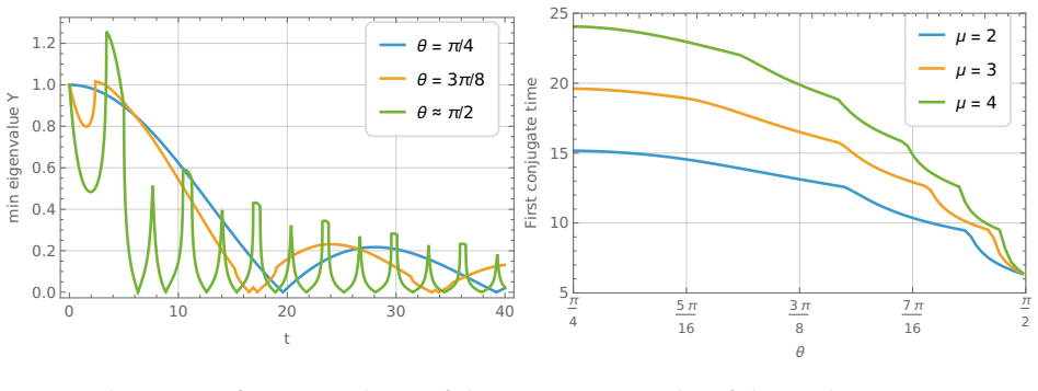
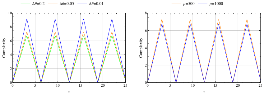
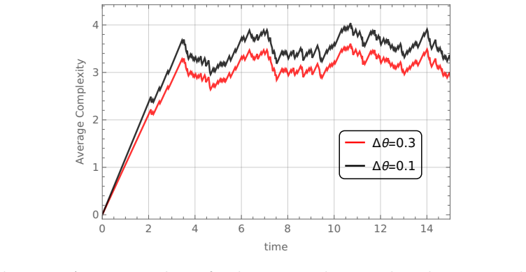
- Approximate analytic solutions for complexity growth exist in the single-qubit case and vary with the penalty hierarchy.
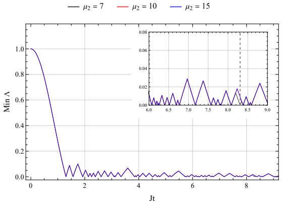
- SYK-type models produce multiple families of conjugate points arising from distinct non-local sectors.
- The occurrence of these conjugate points depends on both the cost hierarchy and the system size.
- Refining the penalty structure supplies a richer description of complexity dynamics.
Where Pith is reading between the lines
- The multi-penalty construction could be applied to model gate costs in physical hardware where locality affects implementation expense.
- It may link complexity geometry more directly to other quantum resource theories that already distinguish local and non-local operations.
- Numerical integration of the modified Jacobi equation in small systems would test the predicted scaling of conjugate points with penalty values.
Load-bearing premise
A hierarchy of penalties can be assigned to directions of different non-locality while preserving right-invariance of the complexity metric.
What would settle it
A calculation for the single-qubit system in which the approximate analytic solutions for complexity growth fail to satisfy the modified Euler-Arnold equation.
Figures


read the original abstract
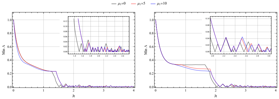
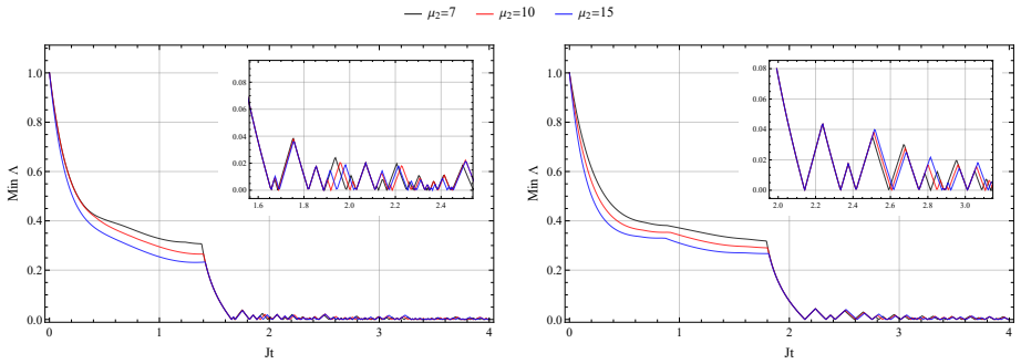
We investigate Nielsen's geometric approach to quantum complexity in the presence of multiple cost factors, extending the standard framework where a single penalty distinguishes easy from hard directions of the group manifold. By introducing a hierarchy of penalties associated with different degrees of non-locality, we develop a generalized right-invariant complexity geometry and analyze its implications for geodesic evolution. We derive the modified Euler-Arnold and Jacobi equations and study how multiple cost factors reshape the structure and scaling of conjugate points, where geodesic optimality breaks down. The formalism is illustrated in two settings: a single-qubit system with two cost factors, where we derive approximate analytic solutions for the complexity growth and its dependence on penalty hierarchies, and SYK-type models, where we analyze both free and chaotic regimes. In these many-body systems, we show that distinct non-local sectors generate multiple families of conjugate points whose occurrence depends on both the cost hierarchy and the system size. Our results highlight how refining the penalty structure provides a richer and more realistic description of quantum complexity and its dynamical behavior.
Editorial analysis
A structured set of objections, weighed in public.
Referee Report
Summary. The paper extends Nielsen's geometric formulation of quantum complexity by replacing the single penalty factor with a hierarchy of cost factors that distinguish operators according to their degree of non-locality. It constructs the associated right-invariant Riemannian metric on the unitary group, derives the modified Euler-Arnold and Jacobi equations that govern geodesics and their variations, and analyzes how the hierarchy alters the location and scaling of conjugate points. Concrete illustrations are given for a single-qubit system with two cost factors and for both free and chaotic regimes of SYK-type models, where multiple families of conjugate points appear whose occurrence depends on the penalty ratios and system size.
Significance. If the derivations are correct, the work supplies a technically straightforward but conceptually richer model of complexity geometry that can accommodate realistic distinctions between local and non-local gates. The explicit treatment of conjugate-point families in the SYK setting offers a concrete handle on how penalty structure influences the breakdown of geodesic optimality, which may prove useful for connecting geometric complexity to dynamical features of chaotic many-body systems. The approach remains fully within the standard right-invariant framework, so the technical overhead is modest.
minor comments (3)
- [§3] The abstract states that the modified Euler-Arnold and Jacobi equations are derived, but the main text should include an explicit step-by-step reduction from the left-trivialized geodesic equation to the new form (perhaps in §3) so that readers can verify the precise manner in which the sector-dependent inner product enters the structure constants.
- [single-qubit section] In the single-qubit example, the approximate analytic solutions for complexity growth are presented; it would be helpful to state the regime of validity of the approximation (e.g., small penalty ratios or short times) and to compare the analytic curves against a numerical integration of the geodesic equation.
- [SYK section] The SYK analysis reports that distinct non-local sectors generate multiple families of conjugate points whose occurrence depends on both the cost hierarchy and system size. A brief table or plot summarizing the leading conjugate-point times as functions of the penalty ratios for N=8,12,16 would make the scaling claim easier to assess.
Simulated Author's Rebuttal
We thank the referee for their positive assessment of the manuscript, including the recognition that the multi-cost-factor extension supplies a technically straightforward yet conceptually richer model, and for the recommendation of minor revision. The report does not enumerate any specific major comments requiring point-by-point replies.
Circularity Check
No significant circularity; derivation is standard Riemannian geometry on Lie groups
full rationale
The paper defines a right-invariant metric by partitioning the Lie algebra basis into sectors of differing non-locality and rescaling the inner product on each sector. Any positive-definite inner product yields a right-invariant Riemannian metric on the group, after which the Euler-Arnold and Jacobi equations follow from the standard left-trivialized geodesic equation with only algebraic modifications to the structure constants. No fitted parameters are relabeled as predictions, no self-citations are invoked as load-bearing uniqueness theorems, and no ansatz is smuggled via prior work. The claimed results on conjugate-point scaling are direct consequences of the chosen metric and system size, not reductions to the inputs by construction. The derivation is therefore self-contained against external benchmarks of Lie-group geometry.
Axiom & Free-Parameter Ledger
Reference graph
Works this paper leans on
-
[1]
Computational complexity,
C. H. Papadimitriou, “Computational complexity,” inEncyclopedia of computer science, pp. 260–265. 2003
2003
-
[2]
Quantum complexity in gravity, quantum field theory, and quantum information science,
S. Baiguera, V. Balasubramanian, P. Caputa, S. Chapman, J. Haferkamp, M. P. Heller, and N. Y. Halpern, “Quantum complexity in gravity, quantum field theory, and quantum information science,”Phys. Rept.1159(2026) 1–77,arXiv:2503.10753 [hep-th]
arXiv 2026
-
[3]
Circuit complexity in interacting QFTs and RG flows,
A. Bhattacharyya, A. Shekar, and A. Sinha, “Circuit complexity in interacting QFTs and RG flows,”JHEP10(2018) 140,arXiv:1808.03105 [hep-th]
Pith/arXiv arXiv 2018
-
[4]
Post-Quench Evolution of Complexity and Entanglement in a Topological System,
T. Ali, A. Bhattacharyya, S. Shajidul Haque, E. H. Kim, and N. Moynihan, “Post-Quench Evolution of Complexity and Entanglement in a Topological System,” Phys. Lett. B811(2020) 135919,arXiv:1811.05985 [hep-th]
arXiv 2020
-
[5]
Quantum Complexity of Time Evolution with Chaotic Hamiltonians,
V. Balasubramanian, M. Decross, A. Kar, and O. Parrikar, “Quantum Complexity of Time Evolution with Chaotic Hamiltonians,”JHEP01(2020) 134,arXiv:1905.05765 [hep-th]. 32
arXiv 2020
-
[6]
Complexity growth in integrable and chaotic models,
V. Balasubramanian, M. DeCross, A. Kar, Y. Li, and O. Parrikar, “Complexity growth in integrable and chaotic models,”JHEP07(2021) 011,arXiv:2101.02209 [hep-th]
arXiv 2021
-
[7]
Bounds on quantum evolution complexity via lattice cryptography,
B. Craps, M. De Clerck, O. Evnin, P. Hacker, and M. Pavlov, “Bounds on quantum evolution complexity via lattice cryptography,”SciPost Phys.13no. 4, (2022) 090, arXiv:2202.13924 [quant-ph]
arXiv 2022
-
[8]
Quantum Many-Body Systems in Thermal Equilibrium,
A. M. Alhambra, “Quantum Many-Body Systems in Thermal Equilibrium,”PRX Quantum4no. 4, (2023) 040201,arXiv:2204.08349 [quant-ph]
arXiv 2023
-
[9]
Quantum complexity and topological phases of matter,
P. Caputa and S. Liu, “Quantum complexity and topological phases of matter,”Phys. Rev. B106no. 19, (2022) 195125,arXiv:2205.05688 [hep-th]
arXiv 2022
-
[10]
Integrability and complexity in quantum spin chains,
B. Craps, M. De Clerck, O. Evnin, and P. Hacker, “Integrability and complexity in quantum spin chains,”SciPost Phys.16no. 2, (2024) 041,arXiv:2305.00037 [quant-ph]
arXiv 2024
-
[11]
Quantitative approaches to information recovery from black holes,
V. Balasubramanian and B. Czech, “Quantitative approaches to information recovery from black holes,”Class. Quant. Grav.28(2011) 163001,arXiv:1102.3566 [hep-th]
Pith/arXiv arXiv 2011
-
[12]
L. Susskind, “Entanglement is not enough,”Fortsch. Phys.64(2016) 49–71, arXiv:1411.0690 [hep-th]
Pith/arXiv arXiv 2016
-
[13]
Holographic Complexity Equals Bulk Action?,
A. R. Brown, D. A. Roberts, L. Susskind, B. Swingle, and Y. Zhao, “Holographic Complexity Equals Bulk Action?,”Phys. Rev. Lett.116no. 19, (2016) 191301, arXiv:1509.07876 [hep-th]
Pith/arXiv arXiv 2016
-
[14]
Circuit complexity in quantum field theory,
R. Jefferson and R. C. Myers, “Circuit complexity in quantum field theory,”JHEP10 (2017) 107,arXiv:1707.08570 [hep-th]
Pith/arXiv arXiv 2017
-
[15]
A Universal Operator Growth Hypothesis,
D. E. Parker, X. Cao, A. Avdoshkin, T. Scaffidi, and E. Altman, “A Universal Operator Growth Hypothesis,”Phys. Rev. X9no. 4, (2019) 041017,arXiv:1812.08657 [cond-mat.stat-mech]
arXiv 2019
-
[16]
Path integral optimization as circuit complexity,
H. A. Camargo, M. P. Heller, R. Jefferson, and J. Knaute, “Path integral optimization as circuit complexity,”Phys. Rev. Lett.123no. 1, (2019) 011601,arXiv:1904.02713 [hep-th]
Pith/arXiv arXiv 2019
-
[17]
On the complexity of quantum field theory,
T. W. Grimm and M. van Vliet, “On the complexity of quantum field theory,”JHEP06 (2025) 215,arXiv:2410.23338 [hep-th]
arXiv 2025
-
[18]
A geometric approach to quantum circuit lower bounds,
M. A. Nielsen, “A geometric approach to quantum circuit lower bounds,”Quant. Inf. Comput.6no. 3, (2006) 213–262,arXiv:quant-ph/0502070
Pith/arXiv arXiv 2006
-
[19]
Quantum Computation as Geometry,
M. A. Nielsen, M. R. Dowling, M. Gu, and A. C. Doherty, “Quantum Computation as Geometry,”Science311no. 5764, (2006) 1133–1135,arXiv:quant-ph/0603161
Pith/arXiv arXiv 2006
-
[20]
The geometry of quantum computation,
M. R. Dowling and M. A. Nielsen, “The geometry of quantum computation,”Quant. Inf. Comput.8no. 10, (2008) 0861–0899,arXiv:quant-ph/0701004
Pith/arXiv arXiv 2008
-
[21]
Complexity geometry of a single qubit,
A. R. Brown and L. Susskind, “Complexity geometry of a single qubit,”Phys. Rev. D 100no. 4, (2019) 046020,arXiv:1903.12621 [hep-th]. 33
arXiv 2019
-
[22]
Toward a Definition of Complexity for Quantum Field Theory States,
S. Chapman, M. P. Heller, H. Marrochio, and F. Pastawski, “Toward a Definition of Complexity for Quantum Field Theory States,”Phys. Rev. Lett.120no. 12, (2018) 121602,arXiv:1707.08582 [hep-th]
Pith/arXiv arXiv 2018
-
[23]
Quantum Complexity and Negative Curvature,
A. R. Brown, L. Susskind, and Y. Zhao, “Quantum Complexity and Negative Curvature,”Phys. Rev. D95no. 4, (2017) 045010,arXiv:1608.02612 [hep-th]
Pith/arXiv arXiv 2017
-
[24]
Geometry of quantum complexity,
R. Auzzi, S. Baiguera, G. B. De Luca, A. Legramandi, G. Nardelli, and N. Zenoni, “Geometry of quantum complexity,”Phys. Rev. D103no. 10, (2021) 106021, arXiv:2011.07601 [hep-th]
arXiv 2021
-
[25]
A quantum complexity lower bound from differential geometry,
A. R. Brown, “A quantum complexity lower bound from differential geometry,”Nature Phys.19no. 3, (2023) 401–406,arXiv:2112.05724 [hep-th]
arXiv 2023
-
[26]
Polynomial equivalence of complexity geometries,
A. R. Brown, “Polynomial equivalence of complexity geometries,”Quantum8(2024) 1391
2024
-
[27]
CFT Complexity and Penalty Factors,
S. Baiguera, N. Chagnet, S. Chapman, and O. Shoval, “CFT Complexity and Penalty Factors,”arXiv:2507.22118 [hep-th]
-
[28]
A relation between krylov and nielsen complexity,
B. Craps, O. Evnin, and G. Pascuzzi, “A relation between krylov and nielsen complexity,”Phys. Rev. Lett.132(Apr, 2024) 160402. https://link.aps.org/doi/10.1103/PhysRevLett.132.160402
-
[29]
B. Craps, O. Evnin, and G. Pascuzzi, “Multiseed krylov complexity,”Phys. Rev. Lett. 134(Feb, 2025) 050402. https://link.aps.org/doi/10.1103/PhysRevLett.134.050402
-
[30]
Todorov,Optimal control theory
E. Todorov,Optimal control theory. MIT Press, 2006
2006
-
[31]
V. I. Arnol’d,Mathematical methods of classical mechanics. Springer Science, 2013
2013
-
[32]
Theory of functionals and of integral and integro-differential equations,
V. Volterra, “Theory of functionals and of integral and integro-differential equations,”
-
[33]
Gapless spin fluid ground state in a random, quantum Heisenberg magnet,
S. Sachdev and J. Ye, “Gapless spin fluid ground state in a random, quantum Heisenberg magnet,”Phys. Rev. Lett.70(1993) 3339,arXiv:cond-mat/9212030
Pith/arXiv arXiv 1993
-
[34]
Quantum statistical mechanics of the Sachdev-Ye-Kitaev model and charged black holes,
S. Sachdev, “Quantum statistical mechanics of the Sachdev-Ye-Kitaev model and charged black holes,”Int. J. Mod. Phys. B38no. 32, (2024) 2430003, arXiv:2304.13744 [cond-mat.str-el]
arXiv 2024
-
[35]
Quantum chaos in the sparse SYK model,
P. Orman, H. Gharibyan, and J. Preskill, “Quantum chaos in the sparse SYK model,” JHEP02(2025) 173,arXiv:2403.13884 [hep-th]. 34
arXiv 2025
discussion (0)
Sign in with ORCID, Apple, or X to comment. Anyone can read and Pith papers without signing in.