REVIEW 4 major objections 4 minor 2 cited by
Predictive posterior sampling from non-stationnary Gaussian process priors via Diffusion models with application to climate data
T0 review · 4 major / 4 minor · reviewed 2026-08-07 · deepseek-v4-flash
Pith's one-line read The paper claims that a diffusion model trained only on realizations of a non-stationary Gaussian random field prior can be conditioned, without retraining, to sample the intractable predictive posterior, and that the resulting…
desk verdict A useful, transparent paper on DGM surrogates for non-stationary GP priors, but the posterior fidelity claim for the full 38-parameter prior rests on an untested extrapolation from a simplified 3-parameter case where the authors themselves admit miscalibration. read the letter →
The pith
A machine-rendered reading of the paper's core claim, the machinery that carries it, and where it could break.
The reading
What carries the argument
The load-bearing mechanism is the denoising diffusion model as a surrogate for the SPDE-based Gaussian random field. Fields are drawn as $X = C^{-1/2}\gamma(S)W$ on a 256×256 grid, where $C$ and $S$ come from a finite-element discretization of the Laplace–Beltrami operator under a spatially varying metric; this spectral structure gives the GP its local anisotropies and lets the denoiser be evaluated against the theoretical floor $\sigma^{2\nu/(\nu+1)}$. Posterior sampling then runs MGDM, a training-free guidance sampler that alternates midpoint noise prediction with data-consistency corrections, so the observations enter at inference time only. The paper's validations use Max-SW and C2ST to compare generated and true distributions, and CRPS and energy score on the real-data experiment.
What would settle it
Take one SSTA case or a synthetic draw from the full prior, run a long Metropolis–Hastings chain on the full 38-parameter prior using the Vecchia likelihood as a reference, and compare its posterior samples to MGDM's with Max-SW over the same 216 slices; if the distance is comparable to the gaps between MGDM and MCMC in Table 2, the claim that MGDM is faithful for the full prior collapses.
Extended reading notes
Core claim
In the paper's own terms, the contribution is a two-step recipe: generate realizations from a locally anisotropic Gaussian random field prior defined through an SPDE on a Riemannian domain; train a denoising diffusion model on those realizations so that its learned distribution is a surrogate for the GP prior; then sample the predictive posterior by applying midpoint guidance (MGDM), a training-free conditioning method, to that surrogate. The paper validates the surrogate by showing the trained denoiser's error follows the optimal scaling $\sigma^{2\nu/(\nu+1)}$ predicted by spectral theory, and by reporting Max-SW and classifier two-sample distances between generated and held-out fields that are small though not exactly zero. It validates posterior sampling by comparing MGDM, DPS, and MGPS against MCMC on a simplified three-parameter globally anisotropic prior, where MGDM systematically gives the lowest Max-SW. On the full non-stationary prior and real SSTA data, MGDM's posterior predictive distributions achieve lower CRPS and energy scores than Vecchia-based MCMC and PriorVAE on all tested cases.
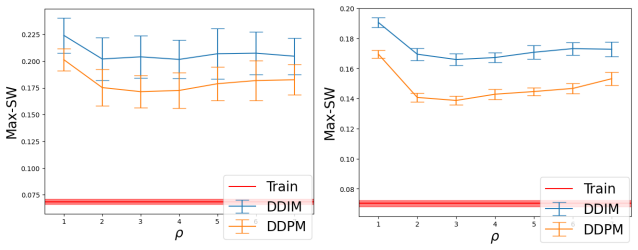
Load-bearing premise
The method's faithfulness on real data rests on the assumption that MGDM remains accurate for the full 38-parameter spatially varying prior, because it is validated against exact MCMC only on a reduced 3-parameter globally anisotropic prior.
Editorial extensions
If this is right
- Once the DGM is trained, generating a posterior sample takes minutes on a GPU, versus hundreds to thousands of minutes for MCMC with Vecchia approximations at comparable observation counts.
- The same trained prior can be fine-tuned to a different parameter distribution over the GP in a handful of epochs, so one base model can serve several spatial priors.
- For cloud-inpainting reconstruction of sea-surface temperature anomalies, the MGDM predictive distribution has lower CRPS and energy score than the two baselines in all three test cases.
- Because the denoiser's error inherits the spectral decay exponent $\nu$, the GP's smoothness controls how well the surrogate can be learned, linking prior regularity to achievable posterior fidelity.
Reading between the lines
- If MGDM's fidelity degrades for spatially varying anisotropy, the CRPS gains over VMCMC on SSTA could be an artifact of the guidance sampler's own regularization rather than evidence that the surrogate posterior matches the true GP posterior; the missing full-prior MCMC benchmark is the test.
- The real-data experiment standardizes each SSTA zone to zero mean and unit variance before applying a centered prior, so the reported posterior is for the standardized field, not the raw temperature anomaly; practitioners must re-embed the mean and scale to interpret the uncertainty.
- The fine-tuning results hint that a single community-trained DGM could be adapted cheaply to new priors, which would shift the cost structure of Bayesian spatial statistics from per-problem MCMC to one amortized training run.
- The spectral error bound suggests a testable extension: train the surrogate at lower resolution and compare the posterior's local anisotropy statistics to the GP's, to separate discretization error from guidance error.
Editorial analysis
A structured set of objections, weighed in public.
Referee Report
Summary. The paper proposes a two-step method for posterior predictive sampling with non-stationary Gaussian process (GP) priors: first train a diffusion generative model (DGM) on realizations of a locally anisotropic GRF prior defined via an SPDE, then use training-free guidance (DPS, MGDM, MGPS) to sample from the posterior conditioned on partial observations. The authors derive an optimal denoising error lower bound (Eq. 5), benchmark the DGM surrogate against held-out GRF samples with Max-SW and C2ST, validate three posterior samplers against an MCMC reference on a reduced global-anisotropy prior (Table 2), and apply the best sampler (MGDM) to sea surface temperature anomaly (SSTA) inpainting, reporting lower CRPS and energy scores than Vecchia-MCMC and PriorVAE (Tables 3 and 7). The central claim is that the DGM surrogate, combined with midpoint guidance, produces posterior samples close to the true GP posterior, yielding state-of-the-art predictions.
Significance. If the central claim were fully supported, the paper would offer a practically valuable and scalable route to Bayesian inference with non-stationary GRF priors that are otherwise intractable, and the explicit link between SPDE-based GRF sampling and DGM training is a useful conceptual contribution. The paper is also transparent: code is provided, the denoiser slope matches the theoretical prediction (Fig. 2), and the fine-tuning experiments (Appendix D.4) show the approach can adapt to different priors. However, the evidence for posterior fidelity is incomplete: the only direct comparison against MCMC uses a simplified prior and shows large distances and acknowledged miscalibration, and the real-data gains are measured only with scoring rules against weak baselines. These gaps are load-bearing for the abstract's claims, so the paper cannot be accepted in its current form.
major comments (4)
- [§4.4, Table 2, Appendix C.4] The validation of MGDM as a posterior sampler is performed only on the reduced 3-parameter 'global anisotropy' prior, while the full prior used in the SSTA experiment has 38 parameters, including 36 spline nodes for spatially varying anisotropy directions. Even on this simplified prior, the Max-SW values between MGDM and the MCMC reference are large in several configurations (e.g., 0.83 for dy=300 unif and 0.74 for dy=355 clust, Table 2), compared with the train-versus-validation Max-SW of 0.069 and the DGM-versus-GRF Max-SW near 0.1 (Table 1). Moreover, Appendix C.4 explicitly states that 'the standard deviation of the errors is not at all the prescribed standard deviation, indicating that all posterior samplers seem not to be calibrated.' This directly undermines the abstract's claim that the issuing distributions are close to their GP counterpart. The authors should either provide a direct validation of the full-prior posterior against a trustworthy reference (e.g., MCMC on a coarse grid or a linear-Gaussian exact posterior) or substantially temper the posterior-fidelity claims.
- [§4.3, Table 1] The C2ST values in Table 1 are above the 5% rejection cutoff of approximately 0.502 (e.g., 0.520 for ResNet101), and the authors themselves state that 'one could safely reject the hypothesis that the two distributions are equal.' While the sensitivity of C2ST in pixel space is acknowledged, this result means the DGM surrogate is statistically distinguishable from the target GRF distribution. Since the posterior is built on this surrogate, the prior approximation error propagates to the posterior; the paper should quantify the effect of this discrepancy on the downstream posterior quantities or provide evidence that it is negligible for the tasks considered.
- [§4.4, SSTA application, Tables 3 and 7] The real-data evaluation reports CRPS and energy score improvements of MGDM over VMCMC and PriorVAE, but there is no reference posterior for the SSTA inverse problem. CRPS and energy score are proper scoring rules, but they reward predictive calibration and sharpness even when the posterior is not the true Bayesian posterior. The baselines are themselves approximate: VMCMC uses a Vecchia approximation on 1000 observations with 16 neighbors (Appendix D.5), and PriorVAE uses a VAE with a simplified likelihood in the NUTS sampler (Appendix D.6). The observed CRPS gains may therefore reflect baseline deficiencies rather than posterior fidelity. A simulated experiment with a known ground-truth field and an exact or highly accurate posterior on the full prior would be needed to support the 'state-of-the-art predictions' claim.
- [§2.2.2, Eq. (4)-(5)] The derivation of the denoising lower bound contains a notational inconsistency that could confuse readers: the text writes 'Trace(Q_σ^{-1})' where the following expression, a sum of (µ_k + σ^{-2})^{-1}, is the trace of Q_σ (since Q_σ = (C^{1/2}γ^{-2}(S)C^{1/2} + σ^{-2}I)^{-1}). The bound itself appears plausible, and the trained denoiser matches the predicted slope in Figure 2, but the displayed equation should be corrected to 'Trace(Q_σ)' to be internally consistent.
minor comments (4)
- [Title and author affiliation] The title contains a typo ('non-stationnary' should be 'non-stationary'), and the affiliation city is spelled 'Fontaineableau' instead of 'Fontainebleau'.
- [§2.2.3] The forward transition kernel is written as 'pt+1|t (xt+1|xt) = N (xt; (σ2 t+1 − σ2 t )I)', which appears to have the variable xt in place of xt+1 in the mean; it should be N(x_{t+1}; x_t, (σ_{t+1}^2 − σ_t^2)I).
- [§4.4] The text says 'DPS[12], MGDM[47], amd MGPS[28]' — 'amd' should be 'and'.
- [Appendix D.1] The phrase 'we plotted as (1 + σ^{-2}) MSE' and the later description of the importance distribution would benefit from a clarifying sentence on how Figure 21 was generated; also the word 'ploted' is misspelled.
Circularity Check
No significant circularity: the DGM posterior approximation is validated against an external MCMC reference and real-data scoring rules, and the self-citations are independent methodological sources rather than premises that already contain the conclusion.
full rationale
The paper's claimed derivation chain is: (i) define a non-stationary GRF prior via the SPDE spectral expansion of Section 2.1; (ii) train a DGM on 300,000 realizations of that prior; (iii) condition the pre-trained DGM with the MGDM guidance algorithm; (iv) evaluate the resulting posterior samples against an MCMC reference on a reduced 3-parameter prior and against CRPS/ES on real SSTA data. None of these steps defines its output in terms of its input by construction. The DGM is fitted to prior draws, but the posterior samples are not forced to equal the GP posterior; that equality is an empirical claim tested with Max-SW and C2ST against held-out data and with Max-SW against MCMC samples. The MCMC benchmark is an external reference (Random Walk Metropolis Hastings on the same simplified prior), and the CRPS/ES on SSTA are scored against real observations, not against training targets or fitted values. The admitted miscalibration in Appendix C.4 and the C2ST values above the 0.502 cutoff are validity and correctness concerns, not circularity: they indicate the approximations are imperfect, but the paper's claims are not true by definition. Self-citations to [53], [39], and [9] supply the SPDE discretization and SMC guidance machinery; these are published, independently usable methods and are not invoked as a 'uniqueness theorem' or as an unverified premise that already contains the conclusion. The choice of rho=3 and the selection of MGDM over DPS/MGPS by validation metrics is model selection, not circularity. Overall, no load-bearing step reduces to its own inputs.
Assumptions & free parameters
free parameters (5)
- prior range a =
U([0.05, 0.3])
- anisotropy ratio min(rho1,rho2)/max(rho1,rho2) =
U([0.1, 1])
- regularity parameter nu =
2
- spline node values for anisotropy direction =
36 iid N(0,1)
- noise schedule shape rho =
3
assumptions (6)
- standard math Spectral theorem for the Laplace-Beltrami operator on compact Riemannian manifolds with Neumann boundary conditions
- standard math Weyl asymptotic law for eigenvalue growth of the discretized Laplacian
- domain assumption The FEM discretization on the expanded domain approximates the continuous SPDE-defined GRF
- ad hoc to paper The DGM surrogate accurately represents the GRF prior distribution
- ad hoc to paper Training-free guidance algorithms (MGDM in particular) sample from the DGM posterior accurately enough
- domain assumption The hand-built prior over GRF parameters is a suitable model for the SSTA data
Cite this review
Pith. "Pith review of Predictive posterior sampling from non-stationnary Gaussian process priors via Diffusion models with application to climate data." pith.science (2026). https://pith.science/paper/AFBTZZXG
@misc{pith2026250524556,
  author       = {Pith},
  title        = {Pith review of: Predictive posterior sampling from non-stationnary Gaussian process priors via Diffusion models with application to climate data},
  year         = {2026},
  howpublished = {\url{https://pith.science/paper/AFBTZZXG}},
  note         = {Machine review of arXiv:2505.24556}
}
read the original abstract
Bayesian models based on Gaussian processes (GPs) offer a flexible framework to predict spatially distributed variables with uncertainty. But the use of nonstationary priors, often necessary for capturing complex spatial patterns, makes sampling from the predictive posterior distribution (PPD) computationally intractable. In this paper, we propose a two-step approach based on diffusion generative models (DGMs) to mimic PPDs associated with non-stationary GP priors: we replace the GP prior by a DGM surrogate, and leverage recent advances on training-free guidance algorithms for DGMs to sample from the desired posterior distribution. We apply our approach to a rich non-stationary GP prior from which exact posterior sampling is untractable and validate that the issuing distributions are close to their GP counterpart using several statistical metrics. We also demonstrate how one can fine-tune the trained DGMs to target specific parts of the GP prior. Finally we apply the proposed approach to solve inverse problems arising in environmental sciences, thus yielding state-of-the-art predictions.
Figures


Figures from the paper (24 more)


Forward citations
Cited by 2 Pith papers
-
Can Deep Generative Models Reproduce Non-Stationary Gaussian Random Fields?
On a known non-stationary Gaussian random field, DDPM and score-SDE reproduce the covariance structure best, flow matching mildly attenuates it, and the VAE largely fails.
-
Neural Conditional Simulation for Complex Spatial Processes
Neural conditional simulation trains a masked diffusion model on unconditional spatial field samples to draw from predictive distributions, demonstrated on Gaussian and Brown–Resnick processes.
Reference graph
Works this paper leans on
-
[1]
J. Ansel, E. Yang, H. He, N. Gimelshein, A. Jain, M. V oznesensky, B. Bao, P. Bell, D. Berard, E. Burovski, G. Chauhan, A. Chourdia, W. Constable, A. Desmaison, Z. DeVito, E. Ellison, W. Feng, J. Gong, M. Gschwind, B. Hirsh, S. Huang, K. Kalambarkar, L. Kirsch, M. Lazos, M. Lezcano, Y . Liang, J. Liang, Y . Lu, C. K. Luk, B. Maher, Y . Pan, C. Puhrsch, M....
arXiv 2024
-
[2]
P. G. Beckman, C. J. Geoga, M. L. Stein, and M. Anitescu. Scalable computations for nonsta- tionary gaussian processes. Statistics and Computing, 33(4):84, Aug. 2023. ISSN 0960-3174, 1573-1375. doi: 10.1007/s11222-023-10252-0
- [3]
- [4]
-
[5]
E. Bingham, J. P. Chen, M. Jankowiak, F. Obermeyer, N. Pradhan, T. Karaletsos, R. Singh, P. A. Szerlip, P. Horsfall, and N. D. Goodman. Pyro: Deep universal probabilistic programming. J. Mach. Learn. Res. , 20:28:1–28:6, 2019. URL http://jmlr.org/papers/v20/18-403. html
work page 2019
-
[6]
S. Bischoff, A. Darcher, M. Deistler, R. Gao, F. Gerken, M. Gloeckler, L. Haxel, J. Kapoor, J. K. Lappalainen, J. H. Macke, G. Moss, M. Pals, F. C. Pei, R. Rapp, A. E. Sa ˘gtekin, C. Schr ¨oder, A. Schulz, Z. Stefanidi, S. Toyota, L. Ulmer, and J. Vetter. A practical guide to sample-based statistical distances for evaluating generative models in science. ...
work page 2024
-
[7]
D. Calvetti and E. Somersalo. Inverse problems: From regularization to bayesian inference. WIREs Computational Statistics , 10(3):e1427, 2018. ISSN 1939-0068. doi: 10.1002/wics. 1427
doi:10.1002/wics 2018
-
[8]
G. Camps-Valls, J. Verrelst, J. Munoz-Mari, V . Laparra, F. Mateo-Jimenez, and J. Gomez- Dans. A survey on gaussian processes for earth-observation data analysis: A comprehensive investigation. IEEE Geoscience and Remote Sensing Magazine, 4(2):58–78, 2016
work page 2016
Show all 72 references
-
[9]
Cardoso, Y
G. Cardoso, Y . J. el idrissi, S. L. Corff, and E. Moulines. Monte Carlo guided Denoising Dif- fusion models for Bayesian linear inverse problems. In The Twelfth International Conference on Learning Representations, 2024
2024
-
[10]
H. Chen, Y . Zhang, X. Cun, M. Xia, X. Wang, C. Weng, and Y . Shan. VideoCrafter2: Overcom- ing data limitations for high-quality video diffusion models. In Proceedings of the IEEE/CVF Conference on Computer Vision and Pattern Recognition, pages 7310–7320, 2024
2024
-
[11]
Y . Chen, O. Wang, R. Zhang, E. Shechtman, X. Wang, and M. Gharbi. Image neural field diffusion models. In 2024 IEEE/CVF Conference on Computer Vision and Pattern Recognition (CVPR), pages 8007–8017, Seattle, W A, USA, June 2024. IEEE. ISBN 979-8-3503-5300-6. doi: 10.1109/CVPR...
2024
-
[12]
Chung, J
H. Chung, J. Kim, M. T. Mccann, M. L. Klasky, and J. C. Ye. Diffusion Posterior Sampling for General Noisy Inverse Problems. In The Eleventh International Conference on Learning Representations, 2023
2023
-
[13]
Chung, D
H. Chung, D. Ryu, M. T. McCann, M. L. Klasky, and J. C. Ye. Solving 3D inverse prob- lems using pre-trained 2D diffusion models. In Proceedings of the IEEE/CVF Conference on Computer Vision and Pattern Recognition, pages 22542–22551, 2023. 11
2023
-
[14]
C. R. Crawford. A Stable Generalized Eigenvalue Problem. SIAM Journal on Numerical Analysis, 13(6):854–860, Dec. 1976. ISSN 0036-1429, 1095-7170. doi: 10.1137/0713067. URL http://epubs.siam.org/doi/10.1137/0713067
1976 doi
-
[15]
Daras, H
G. Daras, H. Chung, C.-H. Lai, Y . Mitsufuji, J. C. Ye, P. Milanfar, A. G. Dimakis, and M. Del- bracio. A survey on diffusion models for inverse problems. CoRR, 2024
2024
-
[16]
De Oliveira and Z
V . De Oliveira and Z. Han. On information about covariance parameters in gaussian mat ´ern random fields. Journal of Agricultural, Biological and Environmental Statistics , 27(4):690– 712, 2022
2022
-
[17]
Dhariwal and A
P. Dhariwal and A. Nichol. Diffusion models beat gans on image synthesis.Advances in neural information processing systems, 34:8780–8794, 2021
2021
-
[18]
P. J. Diggle, J. A. Tawn, and R. A. Moyeed. Model-based geostatistics. Journal of the Royal Statistical Society Series C: Applied Statistics, 47(3):299–350, 1998
1998
-
[19]
Durmus and E
A. Durmus and E. Moulines. Nonasymptotic convergence analysis for the unadjusted Langevin algorithm. The Annals of Applied Probability, 27(3):1551–1587, 2017
2017
-
[20]
M. Elad, B. Kawar, and G. Vaksman. Image denoising: The deep learning revolution and beyond—a survey paper. SIAM Journal on Imaging Sciences, 16(3):1594–1654, 2023
2023
-
[21]
A. E. Gelfand and S. Banerjee. Bayesian modeling and analysis of geostatistical data. Annual review of statistics and its application, 4(1):245–266, 2017
2017
-
[22]
Gneiting, L
T. Gneiting, L. I. Stanberry, E. P. Grimit, L. Held, and N. A. Johnson. Assessing probabilistic forecasts of multivariate quantities, with an application to ensemble predictions of surface winds. Test, 17:211–235, 2008
2008
-
[23]
D. Guo, Y . Wu, S. S. Shitz, and S. Verd ´u. Estimation in gaussian noise: Properties of the minimum mean-square error. IEEE Transactions on Information Theory , 57(4):2371–2385, Apr. 2011. ISSN 0018-9448, 1557-9654. doi: 10.1109/tit.2011.2111010
2011
-
[24]
Han and V
Z. Han and V . De Oliveira. Default priors for the smoothness parameter in gaussian mat ´ern random fields. Bayesian Analysis, 1(1):1–25, 2024
2024
-
[25]
J. Ho, A. Jain, and P. Abbeel. Denoising diffusion probabilistic models. In Advances in Neural Information Processing Systems, volume 33, pages 6840–6851, 2020
2020
-
[26]
Hoffman and A
M. Hoffman and A. Gelman. The No-U-Turn Sampler: Adaptively Setting Path Lengths in Hamiltonian Monte Carlo. Journal of Machine Learning Research, 15, Nov. 2011
2011
-
[27]
Huang, L
H. Huang, L. R. Blake, M. Katzfuss, and D. M. Hammerling. Nonstationary spatial modeling of massive global satellite data. Journal of Computational and Graphical Statistics , pages 1–14, 2025
2025
-
[28]
Janati, B
Y . Janati, B. Moufad, A. Durmus, E. Moulines, and J. Olsson. Divide-and-conquer posterior sampling for denoising diffusion priors. Advances in Neural Information Processing Systems, 37:97408–97444, Dec. 2024
2024
-
[29]
Jordan, F
A. Jordan, F. Kr ¨uger, and S. Lerch. scoringRules: Scoring Rules for Parametric and Simulated Distribution Forecasts, 2022. URL https://CRAN.R-project.org/package= scoringRules. R package version 1.0.2
2022
-
[30]
Kadkhodaie, F
Z. Kadkhodaie, F. Guth, E. P. Simoncelli, and S. Mallat. Generalization in diffusion models arises from geometry-adaptive harmonic representation. In The Twelfth International Confer- ence on Learning Representations, 2023
2023
-
[31]
Karras, M
T. Karras, M. Aittala, T. Aila, and S. Laine. Elucidating the Design Space of Diffusion-Based Generative Models. In Proc. NeurIPS, 2022
2022
-
[32]
Karras, M
T. Karras, M. Aittala, J. Lehtinen, J. Hellsten, T. Aila, and S. Laine. Analyzing and Improving the Training Dynamics of Diffusion Models, Mar. 2024. 12
2024
-
[33]
Katzfuss and J
M. Katzfuss and J. Guinness. A general framework for vecchia approximations of gaussian processes. Statistical Science, 36(1):124–141, 2021
2021
-
[34]
F. E. Kelvinius, Z. Zhao, and F. Lindsten. Solving linear-gaussian bayesian inverse problems with decoupled diffusion sequential monte carlo, Feb. 2025
2025
-
[35]
D. P. Kingma and J. Ba. Adam: A Method for Stochastic Optimization. In Y . Bengio and Y . LeCun, editors, 3rd International Conference on Learning Representations, ICLR 2015, San Diego, CA, USA, May 7-9, 2015, Conference Track Proceedings, 2015
2015
-
[36]
D. P. Kingma and M. Welling. Auto-encoding variational bayes. ICLR, 2014. URL https: //openreview.net/forum?id=33X9fd2-9FyZd
2014
-
[37]
Kupilik, F
M. Kupilik, F. Witmer, and O. Grill. Bias estimation and downscaling for regional climate models using gaussian process regression. IEEE Access, 2024
2024
-
[38]
Labl ´ee
O. Labl ´ee. Spectral theory in Riemannian geometry . EMS Textbooks in mathematics. Euro- pean mathematical society, Z¨urich, 2015. ISBN 978-3-03719-151-4
2015
-
[39]
Lang and M
A. Lang and M. Pereira. Galerkin–chebyshev approximation of gaussian random fields on compact riemannian manifolds. BIT Numerical Mathematics, 63(4):51, 2023
2023
-
[40]
Li and Y
Y . Li and Y . Sun. Efficient estimation of nonstationary spatial covariance functions with appli- cation to high-resolution climate model emulation. Statistica Sinica, 29(3):1209–1231, 2019
2019
-
[41]
Lindgren, H
F. Lindgren, H. Rue, and J. Lindstr ¨om. An explicit link between gaussian fields and gaussian markov random fields: the stochastic partial differential equation approach. Journal of the Royal Statistical Society Series B: Statistical Methodology, 73(4):423–498, 2011
2011
-
[42]
Linhart, A
J. Linhart, A. Gramfort, and P. Rodrigues. L-C2ST: Local diagnostics for posterior approxi- mations in simulation-based inference. Advances in Neural Information Processing Systems , 36:56384–56410, Dec. 2023
2023
-
[43]
Lopez-Paz and M
D. Lopez-Paz and M. Oquab. Revisiting classifier two-sample tests. In International Confer- ence on Learning Representations, Feb. 2017
2017
-
[44]
Lueckmann, J
J.-M. Lueckmann, J. Boelts, D. Greenberg, P. Goncalves, and J. Macke. Benchmarking simulation-based inference. In Proceedings of the 24th International Conference on Artificial Intelligence and Statistics, pages 343–351. PMLR, Mar. 2021
2021
-
[45]
J. E. Matheson and R. L. Winkler. Scoring rules for continuous probability distributions. Man- agement science, 22(10):1087–1096, 1976
1976
-
[46]
MYD35 L2 - MODIS/Aqua Cloud Mask and Spectral Test Results 5-Min L2 Swath 250m and 1km
MODIS Atmosphere Science Team. MYD35 L2 - MODIS/Aqua Cloud Mask and Spectral Test Results 5-Min L2 Swath 250m and 1km. https://ladsweb.modaps.eosdis.nasa. gov/missions-and-measurements/products/MYD35_L2/, 2023
2023
-
[47]
Moufad, Y
B. Moufad, Y . Janati, L. Bedin, A. O. Durmus, R. Douc, E. Moulines, and J. Olsson. Varia- tional diffusion posterior sampling with midpoint guidance. In The Thirteenth International Conference on Learning Representations, Oct. 2024
2024
-
[48]
Nietert, Z
S. Nietert, Z. Goldfeld, R. Sadhu, and K. Kato. Statistical, robustness, and computational guar- antees for sliced wasserstein distances. Advances in Neural Information Processing Systems , 35:28179–28193, Dec. 2022
2022
-
[49]
NOAA Coral Reef Watch Version 3.1 Daily 5km SST Anomalies
NOAA Coral Reef Watch. NOAA Coral Reef Watch Version 3.1 Daily 5km SST Anomalies. https://coralreefwatch.noaa.gov/product/5km/index.php#data_access, 2019
2019
-
[50]
Ongie, A
G. Ongie, A. Jalal, C. A. Metzler, R. G. Baraniuk, A. G. Dimakis, and R. Willett. Deep learning techniques for inverse problems in imaging. IEEE Journal on Selected Areas in Information Theory, 1(1):39–56, May 2020. ISSN 2641-8770. doi: 10.1109/JSAIT.2020.2991563
2020
-
[51]
C. J. Paciorek and M. J. Schervish. Spatial modelling using a new class of nonstationary covariance functions. Environmetrics: The official journal of the International Environmetrics Society, 17(5):483–506, 2006. 13
2006
-
[52]
Pascual, G
S. Pascual, G. Bhattacharya, C. Yeh, J. Pons, and J. Serr `a. Full-band general audio syn- thesis with score-based diffusion. In ICASSP 2023 - 2023 IEEE International Confer- ence on Acoustics, Speech and Signal Processing (ICASSP) , pages 1–5, June 2023. doi: 10.1109/ICASSP49...
2023
-
[53]
Pereira, N
M. Pereira, N. Desassis, and D. Allard. Geostatistics for large datasets on riemannian mani- folds: a matrix-free approach. arXiv preprint arXiv:2208.12501, 2022
2022 arXiv
-
[54]
Petelin, A
D. Petelin, A. Grancharova, and J. Kocijan. Evolving gaussian process models for prediction of ozone concentration in the air. Simulation modelling practice and theory, 33:68–80, 2013
2013
-
[55]
M. D. Risser and D. Turek. Bayesian inference for high-dimensional nonstationary gaussian processes. Journal of Statistical Computation and Simulation, 90(16):2902–2928, 2020
2020
-
[56]
Rombach, A
R. Rombach, A. Blattmann, D. Lorenz, P. Esser, and B. Ommer. High-resolution image syn- thesis with latent diffusion models. In Proceedings of the IEEE/CVF Conference on Computer Vision and Pattern Recognition, pages 10684–10695, 2022
2022
-
[57]
H. Rue, S. Martino, and N. Chopin. Approximate bayesian inference for latent gaussian models by using integrated nested laplace approximations. Journal of the Royal Statistical Society Series B: Statistical Methodology, 71(2):319–392, 2009
2009
-
[58]
H. Rue, A. Riebler, S. H. Sørbye, J. B. Illian, D. P. Simpson, and F. K. Lindgren. Bayesian computing with inla: a review. Annual Review of Statistics and Its Application, 4(1):395–421, 2017
2017
-
[59]
Sang and J
H. Sang and J. Z. Huang. A full scale approximation of covariance functions for large spatial data sets. Journal of the Royal Statistical Society Series B: Statistical Methodology , 74(1): 111–132, 2012
2012
-
[60]
Sawarkar
K. Sawarkar. Deep Learning with PyTorch Lightning: Swiftly Build High-Performance Arti- ficial Intelligence (AI) Models Using Python . Packt Publishing Ltd, Apr. 2022. ISBN 978-1- 80056-927-0
2022
-
[61]
Scarlett, R
J. Scarlett, R. Heckel, M. R. D. Rodrigues, P. Hand, and Y . C. Eldar. Theoretical perspectives on deep learning methods in inverse problems.IEEE Journal on Selected Areas in Information Theory, 3(3):433–453, Sept. 2022. ISSN 2641-8770. doi: 10.1109/JSAIT.2023.3241123
2022
-
[62]
Semenova, Y
E. Semenova, Y . Xu, A. Howes, T. Rashid, S. Bhatt, S. Mishra, and S. Flaxman. PriorV AE: Encoding spatial priors with variational autoencoders for small-area estimation. Journal of the Royal Society, Interface, 19(191):20220094, June 2022. doi: 10.1098/rsif.2022.0094
2022
-
[63]
Semenova, P
E. Semenova, P. Verma, M. Cairney-Leeming, A. Solin, S. Bhatt, and S. Flaxman. PriorCV AE: Scalable MCMC parameter inference with bayesian deep generative modelling, Nov. 2023
2023
-
[64]
Shafieloo, A
A. Shafieloo, A. G. Kim, and E. V . Linder. Gaussian process cosmography. Physical Review D—Particles, Fields, Gravitation, and Cosmology, 85(12):123530, 2012
2012
-
[65]
J. Song, C. Meng, and S. Ermon. Denoising Diffusion Implicit Models. In International Conference on Learning Representations, 2021
2021
-
[66]
J. Song, A. Vahdat, M. Mardani, and J. Kautz. Pseudoinverse-guided diffusion models for inverse problems. In International Conference on Learning Representations, 2023
2023
-
[67]
Y . Song, J. Sohl-Dickstein, D. P. Kingma, A. Kumar, S. Ermon, and B. Poole. Score-Based Generative Modeling through Stochastic Differential Equations. In International Conference on Learning Representations, 2021
2021
-
[68]
P. Vincent. A Connection Between Score Matching and Denoising Autoencoders. Neural Computation, 23(7):1661–1674, 2011
2011
-
[69]
L. Wu, B. L. Trippe, C. A. Naesseth, D. M. Blei, and J. P. Cunningham. Practical and Asymp- totically Exact Conditional Sampling in Diffusion Models. 2023. 14
2023
-
[70]
L. Yang, Z. Zhang, Y . Song, S. Hong, R. Xu, Y . Zhao, W. Zhang, B. Cui, and M.-H. Yang. Diffusion models: A comprehensive survey of methods and applications. ACM Comput. Surv., 56(4):105:1–105:39, Nov. 2023. ISSN 0360-0300. doi: 10.1145/3626235
2023 doi
-
[71]
variables
B. Zhang, W. Chu, J. Berner, C. Meng, A. Anandkumar, and Y . Song. Improving diffusion inverse problem solving with decoupled noise annealing. Corr, Jan. 2024. 15 Appendix Table of Contents A Finite element discretization of random fields 17 B DGM: Additional details and deriv...
2024
-
[72]
mean (standard deviation)
which was run for 1000 steps with learning rate 10−4 and started from a standard Gaussian distribution. The full procedure lasted around 22 minutes running on GPU. D.7 Sea surface temperature anomaly data: details The SSTA data are extracted from the NOAA Coral Reef Watch data...
2025
Reviewed August 7, 2026 · model on record in the stance chip above.
Discussion (0). Continue with ORCID to comment.