REVIEW 2 major objections 4 minor 1 cited by
Continual Release Moment Estimation with Differential Privacy
T0 review · 2 major / 4 minor · reviewed 2026-08-08 · deepseek-v4-flash
Pith's one-line read Joint Moment Estimation (JME) privately releases running first and second moments of a data stream, with the second moment's noise fully covered by the first moment's privacy budget.
desk verdict Genuinely new joint-sensitivity result that delivers 'second moment for free', but the Pareto-dominance claims over IME/CS are proved only under an unproven µ-GDP identification and overreach as stated. read the letter →
The pith
A machine-rendered reading of the paper's core claim, the machinery that carries it, and where it could break.
The reading
What carries the argument
The matrix mechanism with workload matrices A1, A2 and noise shaping matrices C1, C2, together with the joint sensitivity function sens²_λ(C1, C2) = sup_{X∼X'} [‖C1(X−X')‖²_F + λ‖C2(X•X − X'•X')‖²_F]. Lemma 3.5 evaluates this function in closed form for norm-decreasing C1, C2; choosing λ = ‖C1‖²₁→₂ / (c_d ζ² ‖C2‖²₁→₂) with c_d = 8/(11+5√5) for d=1 and c_d=2 for d≥2 makes the joint sensitivity collapse to the first-moment sensitivity 2ζ‖C1‖₁→₂. This collapse is the mechanism that gives 'second moment privacy for free'.
What would settle it
Take a concrete privacy target such as ε=0.1, δ=10⁻⁶ and compute, with the analytical Gaussian calibration used in the paper, the exact noise variances for JME, IME, and CS; if any setting of the trade-off parameters gives IME or CS a strictly smaller second-moment error at the same first-moment error, Theorems 3.6 and 3.7 are contradicted. A second check: numerically maximize the joint sensitivity over neighboring streams for random norm-decreasing C1, C2; any value above 2ζ‖C1‖₁→₂ would refute Lemma 3.5.
Extended reading notes
Core claim
The paper's core discovery is a joint sensitivity identity. For noise-shaping matrices C1 and C2, the squared worst-case change under neighboring streams of the pair (C1X, √λ C2(X • X)) equals ζ²‖C1‖²₁→₂ r_d(λζ²‖C2‖²₁→₂ / ‖C1‖²₁→₂), where r_d is a dimension-dependent piecewise function whose value is 4 for the chosen λ. Since the first moment alone has squared sensitivity 4ζ²‖C1‖²₁→₂, JME's choice of λ makes the joint sensitivity exactly the first-moment sensitivity; the second moment is then released with noise already paid for by the first moment. Consequently, JME produces unbiased estimates of both moments with noise levels that are, in the Frobenius norm, the same as if only the first moment were estimated. The paper further proves that λ-JME Pareto-dominates IME and CS, and that for diagonal-only second moments (as in Adam) the sensitivity is unchanged.
Load-bearing premise
The Pareto-dominance proofs of Theorems 3.6 and 3.7 rely on identifying (ε,δ)-DP with μ-GDP for a specific μ, an equivalence that is not proven and is not generally exact; if this identification fails, the stated dominance for all ε and δ may not hold.
Editorial extensions
If this is right
- Any workload expressible by a lower-triangular matrix—prefix sums, exponential averages, sliding windows—can privately release the second moment at the same noise level as the first moment alone.
- λ-JME offers a strictly better privacy-error trade-off than both independent moment estimation and concatenate-and-split, for any ε and δ.
- In the high-privacy regime, JME's covariance estimation error grows like σ⁴H_{n,2} while post-processing grows like σ⁴H_{n,1}=O(σ⁴ log n), so JME's advantage widens as the stream length n increases.
- DP-Adam with JME matches or beats post-processing-based DP-Adam in high-privacy, small-batch training, while debiased post-processing remains competitive in low-privacy settings.
Reading between the lines
- The free λ parameter in λ-JME could be tuned to minimize a specific downstream loss (e.g. classification error or KL divergence) instead of the worst-case Frobenius error, which may improve practical performance beyond the reported results.
- The same joint-sensitivity technique might extend to other nonlinear features beyond x⊗x, such as third-order moments or kernel features, whenever a similar r_d(λ) bound can be proven; this would give 'privacy for free' for those features too.
- The paper's own low-privacy analysis suggests a hybrid strategy could be optimal: use debiased post-processing when the noise variance is small and JME when it is large, switching based on σ.
Editorial analysis
A structured set of objections, weighed in public.
Referee Report
Summary. The paper proposes Joint Moment Estimation (JME), a method for privately releasing running estimates of the first and second moments of a data stream under continual observation. JME uses the matrix mechanism with two noise-shaping matrices and a joint sensitivity analysis. The main theoretical claim is that by choosing a scaling parameter λ appropriately, the sensitivity of the joint first-plus-second-moment query equals the sensitivity of the first-moment query alone, so the second moment can be estimated without additional privacy cost. The paper presents utility bounds (Theorem 3.3), compares JME to independent moment estimation (IME), concatenate-and-split (CS), and post-processing (PP), and applies the method to private Gaussian density estimation and DP-Adam.
Significance. If correct, the privacy-for-free observation is a genuinely useful contribution: it shows that the second moment can be added to a continual-release pipeline at no extra noise cost, contrary to what composition-based reasoning would suggest. The matrix-mechanism formulation is flexible. The paper also provides exact bias expressions for PP and compares debiased variants. However, the advertised Pareto-dominance over IME and CS (Theorems 3.6, 3.7) currently rests on an informal and unproven identification of (ε,δ)-DP with μ-GDP, and there is a dimension factor error in the utility bound (Theorem 3.3). These issues are local and fixable, but they affect the strength of the claims as stated.
major comments (2)
- [Section 3, Theorem 3.3, Eq. (4)] Equation (4) states that the expected Frobenius error for the second moment is 2ζ^2√(c_d d) σ_{ε,δ} ||C2||_{1→2} ||A2 C2^{-1}||_F. The proof in Appendix A.2 (Eqs. (25)–(26)) yields √(c_d) d instead of √(c_d d). Combining σ = 2ζ σ_{ε,δ} ||C1||_{1→2} and λ* = ||C1||^2 / (c_d ζ^2 ||C2||^2) gives E||S−S_hat||^2_F = 4 c_d d^2 ζ^4 σ_{ε,δ}^2 ||A2 C2^{-1}||_F^2, whose square root is 2ζ^2 d√c_d σ_{ε,δ} ||C2||_{1→2} ||A2 C2^{-1}||_F. Corollary 3.9, Eq. (10), is consistent with the corrected expression (4 c_d d^2 σ^2 ||A2||_F^2 in the trivial factorization). Please correct Eq. (4); the stated dimension dependence is off by a factor of 1/√d and affects any comparison that relies on this bound.
- [Appendix D, proofs of Theorems 3.6 and 3.7] Both proofs open with the sentence 'For the sake of the proof, we assume that (ε,δ)-DP is equivalent to μ-GDP for a specific choice of μ.' This is not proven and is not generally exact: the (ε,δ) guarantee of a Gaussian mechanism is not captured by a single μ, and the budget-splitting identity μ1^2 + μ2^2 = μ^2 used in the proofs is exact only for Gaussian DP composition. Consequently, the statements 'for any ε,δ > 0' in Theorems 3.6 and 3.7 are not established. The central privacy-free result (Theorem 3.2) is unaffected because it is derived directly from a first-principles sensitivity maximization. Please resolve this by (a) proving the Pareto-dominance statements directly under (ε,δ)-DP, or (b) restating Theorems 3.6 and 3.7 explicitly under μ-GDP (or another definition where the composition split is exact), or (c) weakening the claims and adjusting the abstract and introduction accordingly.
minor comments (4)
- [Theorem 4.1] The theorem statement uses Σ and bΣ without defining them explicitly; please state that Σ is the sample covariance matrix and bΣ is the (debiased) JME estimate defined in Section 4.
- [Algorithm 1 (and Algorithm 3)] The notation [C2^{-1} Z2][t,·,·] suggests a 3D array, but Z2 is defined as an n×d^2 matrix; please clarify the reshaping between the n×d^2 noise matrix and the n×d×d representation.
- [Algorithm 2] The line 'λ, sλ = ·Joint-sens(Cβ1 , Cβ2 )' contains a stray dot and the variable sλ is not subsequently defined; please clean up the pseudocode.
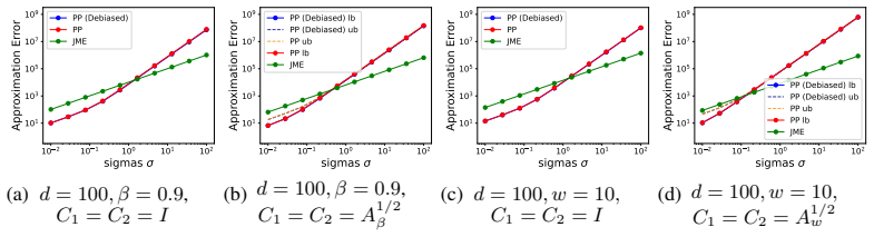
- [Figure 1 caption] The caption refers to 'λ-JME with λ' but does not specify the λ values used in the figure; please state the range or exact values, or clarify that λ is swept.
Circularity Check
No significant circularity: JME's privacy-for-free claim follows from a derived joint-sensitivity bound, not from a fitted input; the unproven mu-GDP identification in Theorems 3.6/3.7 is a rigor gap, not a circular step.
full rationale
The paper's central claim—that JME privately estimates the second moment with no additional privacy cost—is derived from Definition 3.4 and Lemma 3.5, which solve an explicit maximization problem (Problem 1) over neighboring inputs. The scaling parameter lambda is then set analytically to the threshold c_d where r_d(c_d)=4, making the joint sensitivity exactly 2*zeta*||C1||_{1->2}, the first-moment sensitivity. This is a substantive derivation, not a fitted parameter renamed as a prediction. The utility bounds in Theorem 3.3 follow algebraically from the matrix mechanism. The comparisons with IME and CS (Theorems 3.6 and 3.7) are the only load-bearing steps that depend on an extraneous assumption: both proofs state, 'For the sake of the proof, we assume that (epsilon, delta)-DP is equivalent to mu-GDP for a specific choice of mu' (Appendix D). That equivalence is not proven and is generally not exact, so the stated 'for any epsilon, delta > 0' Pareto-dominance is not fully established. This is a correctness or rigor gap, however, not a circularity, because the proofs do not assume the theorem's conclusion and the main sensitivity analysis is independent of the mu-GDP identification. The manuscript also cites prior matrix-mechanism and factorization works, including some by the authors, but these are external published results and are not used to forbid alternatives or to define JME's sensitivity. I find no step where a prediction or first-principles result is equivalent to its inputs by construction.
Assumptions & free parameters
free parameters (2)
- scaling lambda (JME experimental) =
1 (CIFAR-10, Table 3)
- gradient clipping norm =
1 (CIFAR-10)
assumptions (4)
- standard math The Gaussian mechanism calibrated via Balle and Wang achieves (epsilon, delta)-DP for sensitivity-1 queries with variance sigma_{epsilon,delta}^2.
- standard math The matrix mechanism, A(X + C^{-1}Z), is an unbiased private estimate of AX with correlated noise (Li et al.).
- domain assumption C1 and C2 have norm-decreasing columns.
- ad hoc to paper (epsilon, delta)-DP is equivalent to mu-GDP for a specific mu.
Cite this review
Pith. "Pith review of Continual Release Moment Estimation with Differential Privacy." pith.science (2026). https://pith.science/paper/BYW2U7XF
@misc{pith2026250206597,
  author       = {Pith},
  title        = {Pith review of: Continual Release Moment Estimation with Differential Privacy},
  year         = {2026},
  howpublished = {\url{https://pith.science/paper/BYW2U7XF}},
  note         = {Machine review of arXiv:2502.06597}
}
read the original abstract
We propose Joint Moment Estimation (JME), a method for continually and privately estimating both the first and second moments of data with reduced noise compared to naive approaches. JME uses the matrix mechanism and a joint sensitivity analysis to allow the second moment estimation with no additional privacy cost, thereby improving accuracy while maintaining privacy. We demonstrate JME's effectiveness in two applications: estimating the running mean and covariance matrix for Gaussian density estimation, and model training with DP-Adam on CIFAR-10.
Figures


Figures from the paper (4 more)


Forward citations
Cited by 1 Pith paper
-
On Design Principles for Private Adaptive Optimizers
A theoretical and empirical study finds that unbiased second-moment estimates in private Adam can be harmful in high dimensions, and that scale-then-privatize outperforms the alternatives on a small transformer task.
Reference graph
Works this paper leans on
- [1]
-
[2]
D. Achlioptas and F. McSherry. Fast computation of low-rank matrix approximations. Journal of the ACM (JACM), 54(2), 2007
work page 2007
-
[3]
K. Amin, T. Dick, A. Kulesza, A. Munoz, and S. Vassilvitskii. Differentially private covariance estimation. In Conference on Neural Information Processing Systems (NeurIPS), 2019
work page 2019
-
[4]
R. Anil, B. Ghazi, V . Gupta, R. Kumar, and P. Manurangsi. Large-scale differentially private bert. Annual Meeting of the Association for Computational Linguistics (ACL), 2022
work page 2022
-
[5]
B. Balle and Y .-X. Wang. Improving the Gaussian mechanism for differential privacy: Analytical calibration and optimal denoising. In International Conference on Machine Learning (ICML), 2018
work page 2018
-
[6]
A. Blum, C. Dwork, F. McSherry, and K. Nissim. Practical privacy: the SuLQ framework. In International Conference on Management of Data and Symposium on Principles Database and Systems (PODS), 2005
work page 2005
-
[7]
C. A. Choquette-Choo, K. Dvijotham, K. Pillutla, A. Ganesh, T. Steinke, and A. Thakurta. Corre- lated noise provably beats independent noise for differentially private learning. In International Conference on Learning Representations (ICLR), 2024. 10
work page 2024
-
[8]
C. A. Choquette-Choo, A. Ganesh, R. McKenna, H. B. McMahan, J. K. Rush, A. G. Thakurta, and X. Zheng. (Amplified) banded matrix factorization: A unified approach to private training. In Conference on Neural Information Processing Systems (NeurIPS), 2023
work page 2023
Show all 57 references
-
[9]
C. A. Choquette-Choo, H. B. McMahan, K. Rush, and A. Thakurta. Multi-epoch matrix factorization mechanisms for private machine learning. In International Conference on Machine Learning (ICML), 2023
2023
-
[10]
Denisov, H
S. Denisov, H. B. McMahan, J. Rush, A. Smith, and G. A. Thakurta. Improved Differential Privacy for SGD via optimal private linear operators on adaptive streams. In Conference on Neural Information Processing Systems (NeurIPS), 2022
2022
-
[11]
J. C. Duchi, M. I. Jordan, and M. J. Wainwright. Local privacy and statistical minimax rates. In Symposium on Foundations of Computer Science (FOCS), 2013
2013
-
[12]
K. D. Dvijotham, H. B. McMahan, K. Pillutla, T. Steinke, and A. Thakurta. Efficient and near-optimal noise generation for streaming differential privacy. In Symposium on Foundations of Computer Science (FOCS), 2024
2024
-
[13]
Dwork, M
C. Dwork, M. Naor, T. Pitassi, and G. N. Rothblum. Differential privacy under continual observation. In Symposium on Theory of Computing (STOC), 2010
2010
-
[14]
Dwork and A
C. Dwork and A. Roth. The algorithmic foundations of differential privacy. Foundations and Trends in Theoretical Computer Science, 2014
2014
-
[15]
Dwork, K
C. Dwork, K. Talwar, A. Thakurta, and L. Zhang. Analyze Gauss: optimal bounds for privacy- preserving principal component analysis. In Symposium on Theory of Computing (STOC) , 2014
2014
-
[16]
Esteve, E
A. Esteve, E. Boj, and J. Fortiana. Interaction terms in distance-based regression. Communica- tions in Statistics - Theory and Methods, 2009
2009
-
[17]
Fichtenberger, M
H. Fichtenberger, M. Henzinger, and J. Upadhyay. Constant matters: Fine-grained error bound on differentially private continual observation. In International Conference on Machine Learning (ICML), 2023
2023
-
[18]
Henzinger, N
M. Henzinger, N. P. Kalinin, and J. Upadhyay. Binned group algebra factorization for differen- tially private continual counting, 2025. arXiv preprint arXiv:2504.04398
2025 arXiv
-
[19]
Henzinger and J
M. Henzinger and J. Upadhyay. Improved differentially private continual observation using group algebra. In Symposium on Discrete Algorithms (SODA), 2025
2025
-
[20]
Henzinger, J
M. Henzinger, J. Upadhyay, and S. Upadhyay. Almost tight error bounds on differentially private continual counting. In Symposium on Discrete Algorithms (SODA), 2023
2023
-
[21]
Henzinger, J
M. Henzinger, J. Upadhyay, and S. Upadhyay. A unifying framework for differentially private sums under continual observation. In Symposium on Discrete Algorithms (SODA), 2024
2024
-
[22]
Ioffe and C
S. Ioffe and C. Szegedy. Batch normalization: Accelerating deep network training by reducing internal covariate shift. In International Conference on Machine Learning (ICML), 2015
2015
-
[23]
Joseph, M
M. Joseph, M. Ribero, and A. Yu. Privately counting partially ordered data. In International Conference on Learning Representations (ICLR), 2025
2025
-
[24]
Kairouz, B
P. Kairouz, B. McMahan, S. Song, O. Thakkar, A. Thakurta, and Z. Xu. Practical and private (deep) learning without sampling or shuffling. InInternational Conference on Machine Learning (ICML), 2021
2021
-
[25]
Kairouz, S
P. Kairouz, S. Oh, and P. Viswanath. The composition theorem for differential privacy. In International Conference on Machine Learning (ICML), 2015
2015
-
[26]
Kalinin and C
N. Kalinin and C. H. Lampert. Banded square root matrix factorization for differentially private model training. In Conference on Neural Information Processing Systems (NeurIPS), 2024. 11
2024
-
[27]
N. P. Kalinin, R. McKenna, J. Upadhyay, and C. H. Lampert. Back to square roots: An optimal bound on the matrix factorization error for multi-epoch differentially private sgd, 2025. arXiv preprint arXiv:2505.12128
2025
-
[28]
G. Kamath. The broader landscape of robustness in algorithmic statistics. arXiv preprint arXiv:2412.02670, 2024
2024 arXiv
-
[29]
Kamath, A
G. Kamath, A. Mouzakis, and V . Singhal. New lower bounds for private estimation and a generalized fingerprinting lemma. In Conference on Neural Information Processing Systems (NeurIPS), 2020
2020
-
[30]
Kapralov and K
M. Kapralov and K. Talwar. On differentially private low rank approximation. In Symposium on Discrete Algorithms (SODA), 2013
2013
-
[31]
D. P. Kingma and J. Ba. Adam: A method for stochastic optimization. In International Conference on Learning Representations (ICLR), 2015
2015
-
[32]
C. J. Lebeda. Better Gaussian mechanism using correlated noise. In Symposium on Simplicity in Algorithms (SOSA), 2025
2025
-
[33]
C. J. Lebeda and L. Retschmeier. The correlated Gaussian sparse histogram mechanism. arXiv preprint arXiv:2412.10357, 2024
2024 arXiv
-
[34]
C. Li, G. Miklau, M. Hay, A. McGregor, and V . Rastogi. The matrix mechanism: Optimizing linear counting queries under Differential Privacy. International Conference on Very Large Data Bases (VLDB), 2015
2015
-
[35]
X. Li, F. Tramer, P. Liang, and T. Hashimoto. Large language models can be strong differentially private learners. In International Conference on Learning Representations (ICLR), 2022
2022
-
[36]
Mangoubi and N
O. Mangoubi and N. Vishnoi. Re-analyze Gauss: Bounds for private matrix approximation via dyson brownian motion. In Conference on Neural Information Processing Systems (NeurIPS), 2022
2022
-
[37]
Mangoubi and N
O. Mangoubi and N. K. Vishnoi. Private covariance approximation and eigenvalue-gap bounds for complex Gaussian perturbations. In Workshop on Computational Learning Theory (COLT), 2023
2023
-
[38]
H. B. McMahan, K. Pillutla, T. Steinke, and A. Thakurta. Efficient and near-optimal noise generation for streaming differential privacy. In Symposium on Foundations of Computer Science (FOCS), 2024
2024
-
[39]
O. Sheffet. Old techniques in differentially private linear regression. In Algorithmic Learning Theory (ALT), 2019
2019
-
[40]
A. Smith. Privacy-preserving statistical estimation with optimal convergence rates. In Sympo- sium on Theory of Computing (STOC), 2011
2011
-
[41]
Q. Tang, F. Shpilevskiy, and M. Lécuyer. DP-AdamBC: Your DP-Adam is actually DP-SGD (unless you apply bias correction). In Conference on Artificial Intelligence (AAAI), 2024
2024
-
[42]
Upadhyay
J. Upadhyay. The price of privacy for low-rank factorization. In Conference on Neural Information Processing Systems (NeurIPS), 2018
2018
-
[43]
Wilkins, D
A. Wilkins, D. Kifer, D. Zhang, and B. Karrer. Exact privacy analysis of the Gaussian sparse histogram mechanism. Journal of Privacy and Confidentiality, 2024. 12 A Proofs of the main theorems In this section, we provide proofs of Theorem 3.2 and Theorem 3.3 from Section 3 as ...
2024
-
[44]
(21) where rd is specified in (19) or (20), and α2 1 and β2 1 are the squared norms of the first columns of the matrices C1 and C2, respectively. Proof. A straightforward calculation shows sens2 λ(C1, C2) = max i=1,...,n sup ∥x∥≤ζ,∥y∥≤ζ α2 i ∥x − y∥2 2 + λβ2 i ∥x ⊗ x − y ⊗ y∥2...
-
[45]
The proof of the lemma can be found later in the appendix
(29) We apply this lemma recursively to prove that rdiag d (λ) = rdiag 2 (λ) for all d ≥ 2. The proof of the lemma can be found later in the appendix. By combining these lemmas, we conclude the proof of the theorem. 15 B Additional materials Table 1: Common workload matrices f...
-
[46]
// bias-correction bvi = vi/(1 − βi
-
[47]
, θn) Algorithm 3 λ-JME Require: input stream vectors x1,
// bias-correction θi ← θi−1 − α bmi/(√bvi + ϵ) end for Ensure: Θ = (θ1, . . . , θn) Algorithm 3 λ-JME Require: input stream vectors x1, . . . , xn ∈ Rd with ∥xt∥2 ≤ ζ for ζ >0 Require: workload matrices A1 = (at k), A2 = (bt k) ∈ Rn×n Require: noise shaping matrices C1, C2 (l...
-
[48]
If β = − 1 2λ, the objective function is equal to 2 + 2λ + 1 2λ, which concludes the proof
If β = −1, then x = −y and the objective function becomes 4. If β = − 1 2λ, the objective function is equal to 2 + 2λ + 1 2λ, which concludes the proof. Theorem 3.6 (JME vs IME). For any ϵ, δ >0, λ-JME Pareto-dominates IME with respect to the approximation error for the first ...
-
[49]
We begin by selecting indices i and j such that the corresponding components xi, xj from x and yi, yj from y satisfy (x2 i − y2 i )(x2 j − y2 j ) ≥ 0
(29) Proof. We begin by selecting indices i and j such that the corresponding components xi, xj from x and yi, yj from y satisfy (x2 i − y2 i )(x2 j − y2 j ) ≥ 0. We can always find such indices because, by the pigeonhole principle for d ≥ 3, there will be pairs where either b...
-
[50]
Therefore, we look for a solution of the form x = (x1, p 1 − x2
The norm of y, however, can be different. Therefore, we look for a solution of the form x = (x1, p 1 − x2
-
[51]
We now consider the functional in the statement of the lemma in the following form: Lλ(x1, y1, y2) = (x1 + y1)2 + q 1 − x2 1 + y2 2 + λ x2 1 − y2 1 2 + λ 1 − x2 1 − y2 2 2
and y = (−y1, −y2). We now consider the functional in the statement of the lemma in the following form: Lλ(x1, y1, y2) = (x1 + y1)2 + q 1 − x2 1 + y2 2 + λ x2 1 − y2 1 2 + λ 1 − x2 1 − y2 2 2 . (105) We now aim to prove thatsup Lλ(x1, y1, y2) = rdiag 2 (λ) in the constrained d...
-
[52]
= 4 for any λ. From now on, consider y1 ̸= x1; then we can divide by the difference, leading to the system: 1 − 1 − x1y1p 1 − y2 1 p 1 − x2 1 + 4λ (x1 − y1)2 = 0, 1 + 1 + x1y1p 1 − y2 1 p 1 − x2 1 − 4λ (x1 + y1)2 = 0. (110) We consider again the sum and difference to get: 2 + ...
-
[53]
(113) By squaring both sides and subtracting x2 1y2 1, we obtain 4x2 1y2 1 (x2 1 + y2 1)2 (1 − x2 1 − y2
-
[54]
We have found another potentially optimal point y1 = p 1 − x2 1, which we will further investigate
(114) So, either x2 1 + y2 1 = 1, which implies y1 = p 1 − x2 1, or x2 1 + y2 1 = 2x1y1, which implies x1 = y1, which we have already discussed. We have found another potentially optimal point y1 = p 1 − x2 1, which we will further investigate. We now consider it as a function...
-
[55]
(116) = 4(1 − 2x2 1) 1 − 4λx1 p 1 − x2 1 p 1 − x2 1 = 0. (117) The first term gives x1 = 1√ 2, which results in Lλ = 4; otherwise, 4λx1 p 1 − x2 1 = 1, which we can solve by first denoting x2 1 as a new variable in the equation −x4 1 + x2 1 − 1 16λ2 = 0. Using the quadratic fo...
-
[56]
Case II: y2 1 + y2 2 < 1, y1, y2 > 0 (Interior)
Substituting this root back into the function gives us Lλ x∗ 1, q 1 − (x∗ 1)2, x∗ 1 = 2 + 4x∗ 1 q 1 − (x∗ 1)2 | {z } = 1 λ +2λ + 8λ((x∗ 1)4 − (x∗ 1)2)| {z } =− 1 2λ = 2 + 2λ + 1 2λ ≥ 4, (119) which constitutes the function rdiag 2 (λ). Case II: y2 1 + y2 2 < 1, y1, y2 > 0 (Int...
-
[57]
(127) This concludes the proof
= 2 + 2λ + 2x1 − 2λx2 1 ≤ 2 + 2λ + 1 2λ . (127) This concludes the proof. Lemma D.5 (Expected Second Moment Error with PP) . Given the private estimation of the first moment A1(X + C −1 1 Z1), where A1 = B1C1, and the second moment A2(X + C −1 1 Z1) ◦ (X + C −1 1 Z1), where A2...
Reviewed August 8, 2026 · model on record in the stance chip above.
Discussion (0). Continue with ORCID to comment.