REVIEW 4 major objections 8 minor 66 references
SHORES: Serendipitous H-ATLAS-fields Observations of Radio Extragalactic Sources with the ATCA. I: catalog generation and analysis
T0 review · 4 major / 8 minor · reviewed 2026-08-10 · deepseek-v4-flash
Pith's one-line read SHORES builds a 2294-source radio catalog at 2.1 GHz and pushes source counts to 150 microjansky.
desk verdict A useful new 2.1 GHz catalog with a genuinely measured ATCA primary beam to 3 FOV; the 95% completeness claim is provisional until the visual-inspection step is folded into the simulations. read the letter →
The pith
A machine-rendered reading of the paper's core claim, the machinery that carries it, and where it could break.
The reading
What carries the argument
The central machinery is a multiple pencil-beam survey geometry combined with three tools: a directly measured ATCA primary-beam profile (an 8th-order polynomial fit to PKSJ0537-441 observations across the four 512 MHz sub-bands) that extends usable imaging to about three FWHM from each pointing; BLOBCAT source extraction with corrections for peak bias, clean bias, and bandwidth smearing, cross-checked against AEGEAN and PySE; and simulated source injections on the representative field s2242-3241 that define the effective area, completeness, and the SNR $\ge 4.5$ reliability threshold. Together these determine which faint sources are real and how the surveyed area depends on flux density, which is what the source counts and FIR-radio correlation rest on.
What would settle it
Run the same completeness and reliability simulations on a different SHORES shallow field, or on a stack of several fields, injecting sources drawn from a source-count model other than Mancuso et al. (2017); if the recovered 95% completeness flux rises above 0.5 mJy or the false-detection rate at SNR 4.5 exceeds 5%, the quoted catalog statistics would not transfer to the whole survey.
Extended reading notes
Core claim
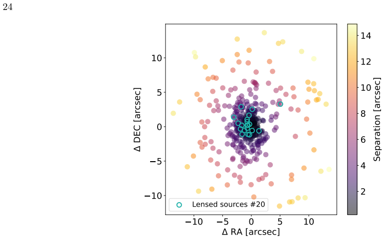
On its own terms, the discovery is that the sub-mJy radio sky at ~2 GHz can be characterized from a set of pointed, serendipitous pencil-beam fields rather than from a dedicated mosaic. By imaging each pointing to three times the ATCA primary-beam FWHM and applying a custom-measured beam correction, the paper obtains a 26-square-degree survey whose effective area grows with flux density; 2294 sources are cataloged at SNR $\ge 4.5$, 81% of them unresolved at 3.2 x 7.2 arcsec. Completeness and reliability, set by simulations on the representative field s2242-3241, reach 95% above 0.5 mJy and at SNR $\ge 4.5$, respectively. The Euclidean source counts at 2.1 GHz extend to 150 microjansky and agree with previous determinations and the Mancuso et al. (2017) model. Cross-matching with H-ATLAS gives 457 counterparts, 394 with enough FIR data for the $q_{\rm FIR}$ FIR-radio correlation, and 20 of the 27 central lensed candidates are detected, doubling the number with radio counterparts from the pilot campaign.
Load-bearing premise
The simulations that set the 95% completeness and reliability assume that the single field s2242-3241 represents the noise and source population of all 27 SHORES fields, and that the injected sources follow the Mancuso et al. (2017) model; the visual inspection step that builds the final catalog is not included in those simulations.
Editorial extensions
If this is right
- Sub-mJy 2.1 GHz source counts are now measured to 150 microjansky over about 26 square degrees, reducing cosmic variance by a factor of $\sqrt{27}$ relative to a single pencil-beam field.
- The 2294-source catalog at 3.2 by 7.2 arcsec resolution, with 81% of sources unresolved, provides a faint radio-source sample for multi-wavelength follow-up and future SKA-era surveys.
- The FIR-radio correlation is extended to ordinary sub-mJy sources, not just lensed candidates, using H-ATLAS counterparts and photometric redshifts for 394 sources.
- Twenty of the 27 central lensed candidates now have radio detections, roughly doubling the number from the pilot campaign and supporting a star-formation origin for their radio emission.
- The measured primary beam correction makes data usable to three times the nominal field of view, improving bright-source statistics and reducing sampling variance in the counts.
Reading between the lines
- If the primary-beam profile is stable across epochs, a similar correction could be applied to archival ATCA observations, turning many historical pointed observations into wide-field source-count measurements.
- The deep SHORES fields, reaching about 8 microjansky, should test whether the Mancuso et al. (2017) model continues to hold below the 150 microjansky limit of this paper.
- The polarization calibration described but not analyzed here could provide a direct test of AGN versus star-formation origin for the sub-mJy sources, with relevance to CMB foreground studies.
Editorial analysis
A structured set of objections, weighed in public.
Referee Report
Summary. The paper presents the SHORES survey, a 2.1 GHz ATCA pencil-beam survey of 27 shallow fields covering ~26 deg² within the H-ATLAS Southern Galactic Field. The authors describe the observations, calibration, imaging, source extraction with three tools (BLOBCAT, AEGEAN, PySE), a custom primary-beam correction measured from dedicated observations, and a final catalog of 2294 sources detected with BLOBCAT at SNR ≥ 4.5. They report 95% completeness above 0.5 mJy and 95% reliability at SNR ≥ 4.5 from simulations on a single representative field, derive 2.1 GHz Euclidean source counts down to 150 μJy after completeness and effective-area corrections, and compare the counts with the Mancuso et al. (2017) model and other surveys. They also cross-match with H-ATLAS to compute the FIR-radio correlation parameter q_FIR for 394 sources and update the status of 20 candidate lensed galaxies.
Significance. If the catalog-level completeness and reliability claims hold, SHORES would provide a valuable new data set at a poorly explored frequency (2.1 GHz) and flux range (sub-mJy to ~1 Jy), with a public catalog, independent cross-checks against NVSS and RACS, and a directly measured ATCA primary beam. The paper's strengths include the multi-tool extraction comparison, the explicit validation against external surveys, the release of the full catalog as supplementary material, and the transparent description of the custom primary-beam and noise-profile corrections. The main significance rests on the faint-end source counts, which are used to test models of the sub-mJy radio population; therefore the completeness correction applied to those counts is the key load-bearing element.
major comments (4)
- [§4.5 and §5] The completeness and reliability simulations validate BLOBCAT extraction on one representative field, but the published catalog is the product of BLOBCAT plus two stages of visual inspection described in §5, which reduced the 2649 SNR ≥ 4.5 detections to the 2294 published sources. The simulations do not include these inspection steps; if any genuine source was removed during inspection, the true completeness of the final catalog is lower than the quoted 95%. The paper does not quantify how many of the 355 removed objects were artifacts versus real sources contaminated by bright neighbors. Because the source counts in §6 are corrected with 1/C(S) derived from these simulations, this issue directly affects the validity of the faint-end counts. Please extend the completeness/reliability analysis to the full catalog-production pipeline, or provide an explicit bound on the number of real sources removed by the visual inspections.
- [§4.4 and §4.5] The completeness simulation is run only on field s2242-3241, chosen because its pixel-histogram distribution is closest to the median of the 27 fields (Figure 10). Table 5 shows that the per-field rms noise varies by about 35% (σ_B from 31 to 46 μJy), and the completeness correction 1/C(S) is largest at the faint fluxes that dominate the 150 μJy counts. The representativeness of s2242-3241 is not validated at the faint end, where source density, confusion, and calibration artifacts could differ between fields. Please run injection tests on at least a few fields spanning the observed σ_B range, or conservatively inflate the completeness uncertainty used in the source-count error budget.
- [§4.5 and §6] The completeness simulations inject sources drawn from the Mancuso et al. (2017) model, and the same model is used as the reference for the derived 2.1 GHz counts in Figure 20. Since several co-authors of the present paper are also authors of Mancuso et al. (2017), the agreement of the corrected counts with that model is not fully independent. The circularity is not absolute—the completeness correction is not forced to fit the model—but a mismatch between the true source population and the injection model would bias C(S) and hence the corrected counts. A concrete test would be to repeat the completeness simulations with an independent source-count model (e.g., one of the other literature counts shown in Figure 20) and report the change in the corrected counts; this should be added.
- [§4.5 and §5] The completeness simulations inject only point sources, while the final catalog contains 376 extended and 62 multi-component sources (§5). Detection efficiency for extended sources at fixed peak SNR is generally lower than for point sources, so the quoted 95% completeness above 0.5 mJy may not apply to the extended subset. Please state explicitly whether the completeness claim applies to the full catalog or only to point sources, and if the latter, provide separate completeness estimates for the extended and multi-component populations.
minor comments (8)
- [§3.1] Typo: "coverign" should be "covering" in the description of leakage calibrator observations.
- [Table 1] The header of Table 1 reads "T able 1"; it should be "Table 1".
- [Abstract and title] The title and abstract contain "A TLAS" and "A TCA", which should be "ATLAS" and "ATCA".
- [§2] The target name "HATLASJ005132.8-01848" appears incomplete; it likely should be "HATLASJ005132.8-301848" or similar.
- [§4.1 and §5] The number of BLOBCAT SNR ≥ 3 detections is inconsistent: Table 2 lists 13662, while §4.1 and §5 state 13688. Please unify these values.
- [§6] The text refers to "2297 SHORES sources" in the counts paragraph, but the catalog has 2294 sources; this appears to be a typo.
- [Figure 15] The left panel label "S=467.7 Jy" should presumably be "467.7 μJy" (or 0.468 mJy), consistent with the 95% completeness threshold quoted in the text.
- [Table 7] The column header "S2.5 2.1GHzdN/dS" is garbled; it should read "S^2.5 dN/dS" with the units correctly formatted.
Circularity Check
Mild circularity: completeness simulations and the model comparison both use the Mancuso et al. (2017) counts; otherwise the catalog derivation is self-contained.
-
other
[Sections 4.5 and 6 (completeness simulations and Fig. 20 comparison)]
"To perform the simulation, we injected 10000 point sources of flux density extracted according to the radio number counts by Mancuso et al. (2017), one at a time, into random positions on the inverse map of s2242-3241 using the Miriad task IMGEN. ... The number of sources per bin of flux have been corrected for the completeness (see Figure 15) and divided by the effective area ... For comparison and reference, we reported the predictions by the Mancuso et al. (2017) model at 2.1 GHz."
The completeness correction C(S) applied to the measured source counts is estimated by injecting fake sources whose flux distribution is exactly the Mancuso et al. (2017) model, and the corrected counts are then displayed against that same model as the reference curve. In finite flux bins, C(S) is a detection probability averaged over the injected model's flux distribution, so the faint-end counts inherit part of the model's shape where the correction is largest (e.g., the 0.15-0.68 mJy bin). Thus the claimed agreement with Mancuso et al. is partly an input-output loop rather than a fully independent test.
full rationale
The core catalog construction is largely self-contained: flux densities come from ATCA observations extracted with BLOBCAT, cross-checked with AEGEAN and PySE and against NVSS and RACS, and the primary-beam correction is measured from a dedicated calibrator observation rather than assumed from prior work. The main circularity concern is confined to the faint-end source-count comparison: the completeness correction is calibrated on injections drawn from Mancuso et al. (2017), and the same model is used as the comparison curve in Fig. 20. Because C(S) is a per-flux detection probability and the real detected counts enter the estimate directly, the corrected counts are not equal to the model by construction; the self-citation is mildly load-bearing but not decisive. I find no self-definitional equations, no fitted parameter renamed as a prediction, and no uniqueness argument imported from the authors' prior work. The SNR>=4.5 threshold is chosen so that the negative-map reliability is 95%, so the phrase '95% reliable' restates the operating point rather than predicts it, which is standard practice and not scored as circular. Separate limitations—completeness/reliability simulations use one representative field and do not include the manual visual-inspection step that pruned the catalog from 2649 to 2294 sources—are real validity gaps, but they are not circularity.
Assumptions & free parameters
free parameters (5)
- Spectral index alpha =
-0.7
- Dust emissivity index beta =
1.5
- Modified blackbody temperature and normalization (per source) =
Free parameters per source
- SNR detection threshold =
4.5
- Rest threshold for extended sources =
2
assumptions (4)
- domain assumption Field s2242-3241 is representative of all 27 SHORES fields for completeness and reliability simulations.
- domain assumption The primary beam response measured on PKSJ0537-441 applies to all SHORES fields.
- domain assumption The Mancuso et al. (2017) source count model describes the true underlying radio source population for simulations.
- domain assumption H-ATLAS SPIRE photometric redshifts are sufficiently accurate for luminosity and qFIR computations.
Cite this review
Pith. "Pith review of SHORES: Serendipitous H-ATLAS-fields Observations of Radio Extragalactic Sources with the ATCA. I: catalog generation and analysis." pith.science (2026). https://pith.science/paper/C3Z7VJME
@misc{pith2026250109662,
  author       = {Pith},
  title        = {Pith review of: SHORES: Serendipitous H-ATLAS-fields Observations of Radio Extragalactic Sources with the ATCA. I: catalog generation and analysis},
  year         = {2026},
  howpublished = {\url{https://pith.science/paper/C3Z7VJME}},
  note         = {Machine review of arXiv:2501.09662}
}
abstract
We introduce the Serendipitous H-ATLAS-fields Observations of Radio Extragalactic Sources (SHORES) multiple pencil beam survey that observed at 2.1 GHz with the Australia Telescope Compact Array (ATCA) 29 fields in total intensity and polarization within the Herschel-ATLAS Southern Galactic Field. This paper presents the observations, calibration and analysis of the 27 shallow fields that cover an overall area of $\sim 26$ square degree with increasing sensitivity towards the phase centers of each pointing according to the ATCA 22 m dish response function, down to $\sigma\lesssim 33\, \mu$Jy. Two additional (deep) fields have been observed to even higher sensitivity. All the SHORES observations have been calibrated to account also for linear polarization. Polarization and deeper field analysis will be presented in future papers. The SHORES shallow-field sample considered in the present paper counts $2294$ sources detected with BLOBCAT to signal-to-noise ratio $SNR\gtrsim 4.5$. Simulations determined that our procedure and final catalog is 95% reliable above $497.5\, \mu$Jy and $95\%$ complete to the $SNR\gtrsim 4.5$ significance level. By exploiting ATCA E-W 6 km configuration we reached resolutions of $3.2\times 7.2$ arcsec, to which level $81\%$ of our sources are unresolved. We determined source counts down to the $150\, \mu$Jy level. For the sources with a counterpart in H-ATLAS, the FIR-radio correlation is calculated and discussed.
Figures


Figures from the paper (20 more)




Reference graph
Works this paper leans on
-
[1]
, " * write output.state after.block = add.period write newline
ENTRY address archivePrefix author booktitle chapter doi edition editor eprint howpublished institution journal key month number organization pages publisher school series title misctitle type volume year version url label extra.label sort.label short.list INTEGERS output.state before.all mid.sentence after.sentence after.block FUNCTION init.state.consts ...
-
[2]
write newline
" write newline "" before.all 'output.state := FUNCTION format.url url empty "" new.block "" url * "" * if FUNCTION format.eprint eprint empty "" archivePrefix empty "" archivePrefix "arXiv" = new.block " " eprint * " " * new.block " " eprint * " " * if if if FUNCTION format.doi doi empty "" " " doi * " " * if FUNCTION format.pid doi empty eprint empty ur...
-
[3]
thebibliography [1] 20pt to REFERENCES 6pt =0pt -12pt 10pt plus 3pt =0pt =0pt =1pt plus 1pt =0pt =0pt -12pt =13pt plus 1pt =20pt =13pt plus 1pt \@M =10000 =-1.0em =0pt =0pt 0pt =0pt =1.0em @enumiv\@empty 10000 10000 `\.\@m \@noitemerr \@latex@warning Empty `thebibliography' environment \@ifnextchar \@reference \@latexerr Missing key on reference command E...
arXiv 2021
-
[4]
2024, Galaxies, 12, 14, 10.3390/galaxies12020014
Behiri , M., Giulietti , M., Galluzzi , V., et al. 2024, Galaxies, 12, 14, 10.3390/galaxies12020014
-
[5]
Bock , D. C. J., Large , M. I., & Sadler , E. M. 1999, , 117, 1578, 10.1086/300786
doi:10.1086/300786 1999
-
[6]
2021, , 500, 22, 10.1093/mnras/staa3218
Bonato , M., Prandoni , I., De Zotti , G., et al. 2021, , 500, 22, 10.1093/mnras/staa3218
-
[7]
2017, , 472, 628, 10.1093/mnras/stx2102
Bonavera , L., Gonz \'a lez-Nuevo , J., De Marco , B., Arg \"u eso , F., & Toffolatti , L. 2017, , 472, 628, 10.1093/mnras/stx2102
-
[8]
2008, , 681, 1129, 10.1086/589324
Bondi , M., Ciliegi , P., Schinnerer , E., et al. 2008, , 681, 1129, 10.1086/589324
doi:10.1086/589324 2008
Show all 66 references
-
[9]
2003, , 403, 857, 10.1051/0004-6361:20030382
Bondi , M., Ciliegi , P., Zamorani , G., et al. 2003, , 403, 857, 10.1051/0004-6361:20030382
2003 doi
-
[10]
2023, , 10.1093/mnras/stad3381
Borsato , E., Marchetti , L., Negrello , M., et al. 2023, , 10.1093/mnras/stad3381
2023 doi
-
[11]
M., Hopkins , A
Boyce , M. M., Hopkins , A. M., Riggi , S., et al. 2023, , 40, e027, 10.1017/pasa.2023.29
2023 doi
-
[12]
H., & Schwab , F
Bridle , A. H., & Schwab , F. R. 1999, in Astronomical Society of the Pacific Conference Series, Vol. 180, Synthesis Imaging in Radio Astronomy II, ed. G. B. Taylor , C. L. Carilli , & R. A. Perley , 371
1999
-
[13]
2018, , 620, A3, 10.1051/0004-6361/201630129
Butler , A., Huynh , M., Delhaize , J., et al. 2018, , 620, A3, 10.1051/0004-6361/201630129
2018 doi
-
[14]
2018, Astronomy and Computing, 23, 92, 10.1016/j.ascom.2018.02.003
Carbone , D., Garsden , H., Spreeuw , H., et al. 2018, Astronomy and Computing, 23, 92, 10.1016/j.ascom.2018.02.003
2018 doi
-
[15]
Condon , J. J. 1992, in American Institute of Physics Conference Series, Vol. 254, Testing the AGN paradigm, ed. S. S. Holt , S. G. Neff , & C. M. Urry , 629--639, 10.1063/1.42217
1992 doi
-
[16]
J., Cotton , W
Condon , J. J., Cotton , W. D., Greisen , E. W., et al. 1998, , 115, 1693, 10.1086/300337
1998 doi
-
[17]
J., Cotton , W
Condon , J. J., Cotton , W. D., Fomalont , E. B., et al. 2012, , 758, 23, 10.1088/0004-637X/758/1/23
2012 doi
-
[18]
2022, , 668, A133, 10.1051/0004-6361/202244452
D'Amato , Q., Prandoni , I., Gilli , R., et al. 2022, , 668, A133, 10.1051/0004-6361/202244452
2022 doi
- [19]
-
[20]
2010, , 18, 1, 10.1007/s00159-009-0026-0
de Zotti , G., Massardi , M., Negrello , M., & Wall , J. 2010, , 18, 1, 10.1007/s00159-009-0026-0
2010 doi
-
[21]
T., et al
Delvecchio , I., Daddi , E., Sargent , M. T., et al. 2021, , 647, A123, 10.1051/0004-6361/202039647
2021 doi
-
[22]
W., Grundy , J
Duchesne , S. W., Grundy , J. A., Heald , G. H., et al. 2024, , 41, e003, 10.1017/pasa.2023.60
2024 doi
-
[23]
2010, , 122, 499, 10.1086/653086
Eales , S., Dunne , L., Clements , D., et al. 2010, , 122, 499, 10.1086/653086
2010 doi
-
[24]
S., Gaensler , B
Farnes , J. S., Gaensler , B. M., & Carretti , E. 2014, , 212, 15, 10.1088/0067-0049/212/1/15
2014 doi
-
[25]
2017, , 465, 4085, 10.1093/mnras/stw3017
Galluzzi , V., Massardi , M., Bonaldi , A., et al. 2017, , 465, 4085, 10.1093/mnras/stw3017
2017 doi
-
[26]
2022, , 511, 1408, 10.1093/mnras/stac145
Giulietti , M., Massardi , M., Lapi , A., et al. 2022, , 511, 1408, 10.1093/mnras/stac145
2022 doi
- [27]
-
[28]
1999, , 305, 297, 10.1046/j.1365-8711.1999.02415.x
Gruppioni , C., Ciliegi , P., Rowan-Robinson , M., et al. 1999, , 305, 297, 10.1046/j.1365-8711.1999.02415.x
1999
-
[29]
2022, , 512, 6104, 10.1093/mnras/stac880
G \"u rkan , G., Prandoni , I., O'Brien , A., et al. 2022, , 512, 6104, 10.1093/mnras/stac880
2022 doi
-
[30]
L., McConnell , D., Thomson , A
Hale , C. L., McConnell , D., Thomson , A. J. M., et al. 2021, , 38, e058, 10.1017/pasa.2021.47
2021 doi
-
[32]
J., Murphy , T., Gaensler , B
Hancock , P. J., Murphy , T., Gaensler , B. M., Hopkins , A., & Curran , J. R. 2012, , 422, 1812, 10.1111/j.1365-2966.2012.20768.x
2012
-
[33]
J., Trott , C
Hancock , P. J., Trott , C. M., & Hurley-Walker , N. 2018, , 35, e011, 10.1017/pasa.2018.3
2018 doi
-
[34]
J., White , R
Helfand , D. J., White , R. L., & Becker , R. H. 2015, , 801, 26, 10.1088/0004-637X/801/1/26
2015 doi
-
[35]
L., Jarvis , M
Heywood , I., Hale , C. L., Jarvis , M. J., et al. 2020, , 496, 3469, 10.1093/mnras/staa1770
2020 doi
-
[36]
J., & Condon , J
Heywood , I., Jarvis , M. J., & Condon , J. J. 2013, , 432, 2625, 10.1093/mnras/stt843
2013 doi
-
[37]
J., Baker , A
Heywood , I., Jarvis , M. J., Baker , A. J., et al. 2016, , 460, 4433, 10.1093/mnras/stw1250
2016 doi
-
[38]
J., Hale , C
Heywood , I., Jarvis , M. J., Hale , C. L., et al. 2022, , 509, 2150, 10.1093/mnras/stab3021
2022 doi
-
[39]
M., Afonso , J., Chan , B., et al
Hopkins , A. M., Afonso , J., Chan , B., et al. 2003, , 125, 465, 10.1086/345974
2003 doi
-
[40]
M., Mobasher , B., Cram , L., & Rowan-Robinson , M
Hopkins , A. M., Mobasher , B., Cram , L., & Rowan-Robinson , M. 1998, , 296, 839, 10.1046/j.1365-8711.1998.01403.x
1998
-
[41]
M., Whiting , M
Hopkins , A. M., Whiting , M. T., Seymour , N., et al. 2015, , 32, e037, 10.1017/pasa.2015.37
2015 doi
-
[42]
J., Duchesne , S
Hurley-Walker , N., Galvin , T. J., Duchesne , S. W., et al. 2022, , 39, e035, 10.1017/pasa.2022.17
2022 doi
-
[43]
J., Magnelli , B., Ibar , E., et al
Ivison , R. J., Magnelli , B., Ibar , E., et al. 2010, , 518, L31, 10.1051/0004-6361/201014552
2010 doi
-
[44]
C., & Thompson , T
Lacki , B. C., & Thompson , T. A. 2010, , 717, 196, 10.1088/0004-637X/717/1/196
2010 doi
-
[45]
A., Chandler , C
Lacy , M., Baum , S. A., Chandler , C. J., et al. 2020, , 132, 035001, 10.1088/1538-3873/ab63eb
2020 doi
-
[46]
S., et al
Lamee , M., Rudnick , L., Farnes , J. S., et al. 2016, , 829, 5, 10.3847/0004-637X/829/1/5
2016 doi
-
[47]
2018, , 857, 22, 10.3847/1538-4357/aab6af
Lapi , A., Pantoni , L., Zanisi , L., et al. 2018, , 857, 22, 10.3847/1538-4357/aab6af
2018 doi
-
[48]
J., Lutz , D., et al
Magnelli , B., Ivison , R. J., Lutz , D., et al. 2015, , 573, A45, 10.1051/0004-6361/201424937
2015 doi
-
[49]
2017, , 842, 95, 10.3847/1538-4357/aa745d
Mancuso , C., Lapi , A., Prandoni , I., et al. 2017, , 842, 95, 10.3847/1538-4357/aa745d
2017 doi
-
[51]
2016, International Journal of Modern Physics D, 25, 1640009, 10.1142/S0218271816400095
Massardi , M., Galluzzi , V., Paladino , R., & Burigana , C. 2016, International Journal of Modern Physics D, 25, 1640009, 10.1142/S0218271816400095
2016 doi
-
[52]
D., Murphy , T., et al
Massardi , M., Ekers , R. D., Murphy , T., et al. 2011, , 412, 318, 10.1111/j.1365-2966.2010.17917.x
2011
-
[53]
L., Lenc , E., et al
McConnell , D., Hale , C. L., Lenc , E., et al. 2020, , 37, e048, 10.1017/pasa.2020.41
2020 doi
-
[54]
M., Ekers , R
Murphy , T., Sadler , E. M., Ekers , R. D., et al. 2010, , 402, 2403, 10.1111/j.1365-2966.2009.15961.x
2010
-
[55]
2017, Submillimeter Array Newsletter, 24, 10
Negrello , M., & Herschel-Atlas Team . 2017, Submillimeter Array Newsletter, 24, 10
2017
-
[56]
P., Marvil , J., Collier , J
Norris , R. P., Marvil , J., Collier , J. D., et al. 2021, , 38, e046, 10.1017/pasa.2021.42
2021 doi
-
[57]
2017, , 602, A5, 10.1051/0004-6361/201629436
Novak , M., Smol c i \'c , V., Delhaize , J., et al. 2017, , 602, A5, 10.1051/0004-6361/201629436
2017 doi
-
[58]
R., McKinley , B., Hurley-Walker , N., et al
Offringa , A. R., McKinley , B., Hurley-Walker , N., et al. 2014, , 444, 606, 10.1093/mnras/stu1368
2014 doi
-
[59]
2020, , 641, A1, 10.1051/0004-6361/201833880
Planck Collaboration , Aghanim , N., Akrami , Y., et al. 2020, , 641, A1, 10.1051/0004-6361/201833880
2020 doi
-
[60]
2000, , 146, 31, 10.1051/aas:2000360
Prandoni , I., Gregorini , L., Parma , P., et al. 2000, , 146, 31, 10.1051/aas:2000360
2000 doi
-
[61]
2018, , 481, 4548, 10.1093/mnras/sty2521
Prandoni , I., Guglielmino , G., Morganti , R., et al. 2018, , 481, 4548, 10.1093/mnras/sty2521
2018 doi
- [62]
-
[63]
Schleicher , D. R. G., & Beck , R. 2013, , 556, A142, 10.1051/0004-6361/201321707
2013 doi
-
[64]
Schober , J., Schleicher , D. R. G., & Klessen , R. S. 2016, , 827, 109, 10.3847/0004-637X/827/2/109
2016 doi
-
[65]
2017, Royal Society Open Science, 4, 170522, 10.1098/rsos.170522
Simpson , C. 2017, Royal Society Open Science, 4, 170522, 10.1098/rsos.170522
2017 doi
-
[66]
2018, , 620, A14, 10.1051/0004-6361/201732336
Smol c i \'c , V., Intema , H., S laus , B., et al. 2018, , 620, A14, 10.1051/0004-6361/201732336
2018 doi
-
[67]
2018, , 618, A29, 10.1051/0004-6361/201732342
Trombetti , T., Burigana , C., De Zotti , G., Galluzzi , V., & Massardi , M. 2018, , 618, A29, 10.1051/0004-6361/201732342
2018 doi
-
[68]
S., & Carilli , C
Yun , M. S., & Carilli , C. 2001, in Astronomical Society of the Pacific Conference Series, Vol. 235, Science with the Atacama Large Millimeter Array, ed. A. Wootten , 351
2001
Reviewed August 10, 2026 · model on record in the stance chip above.
Discussion (0). Continue with ORCID to comment.