Flatland: The Adventures of Gradient Descent with Large Step Sizes
Pith reviewed 2026-06-28 02:10 UTC · model grok-4.3
The pith
Adaptive methods allow gradient descent to use large step sizes while remaining at the edge of stability from the start of training.
A machine-rendered reading of the paper's core claim, the machinery that carries it, and where it could break.
Core claim
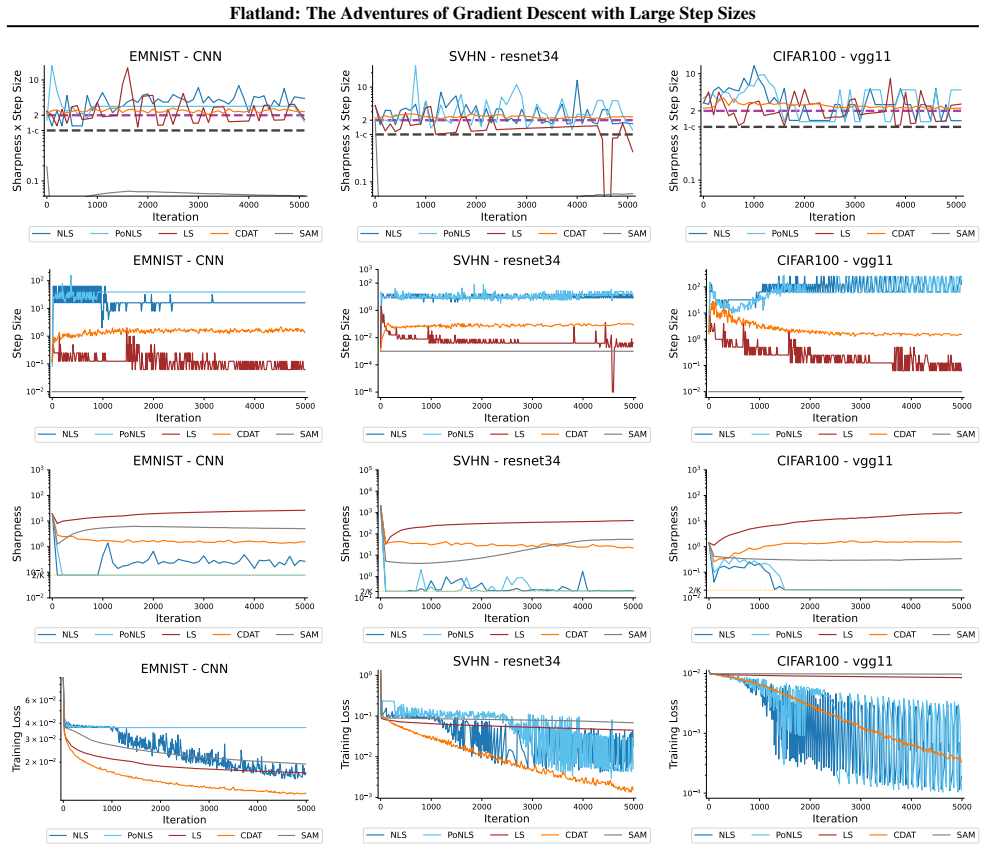
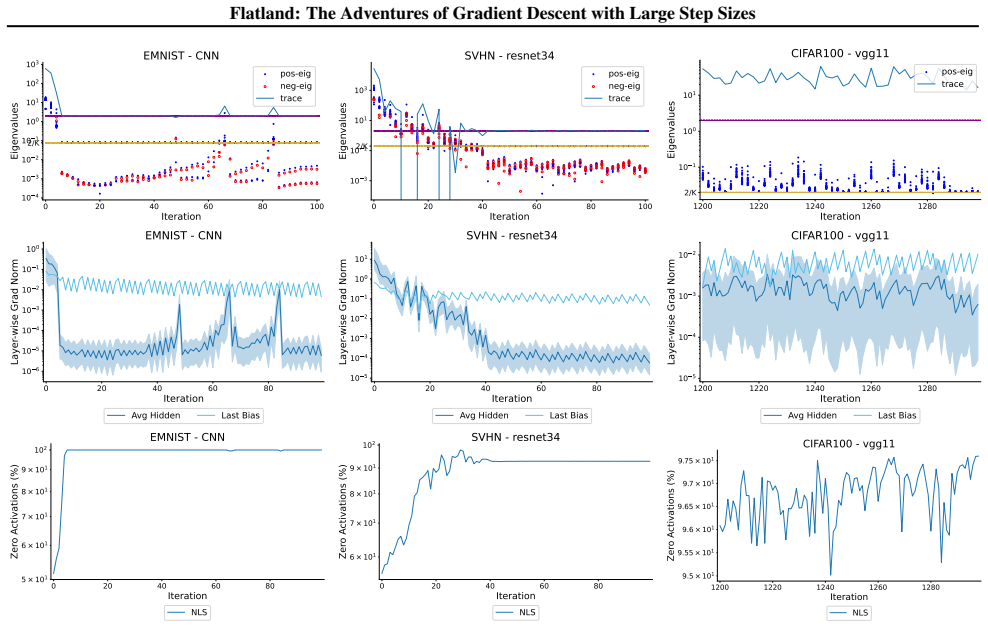
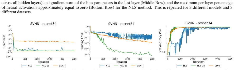
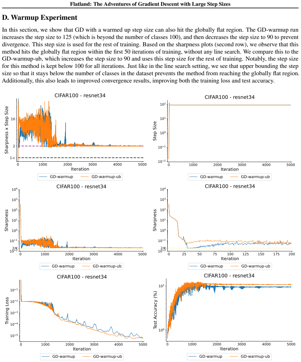
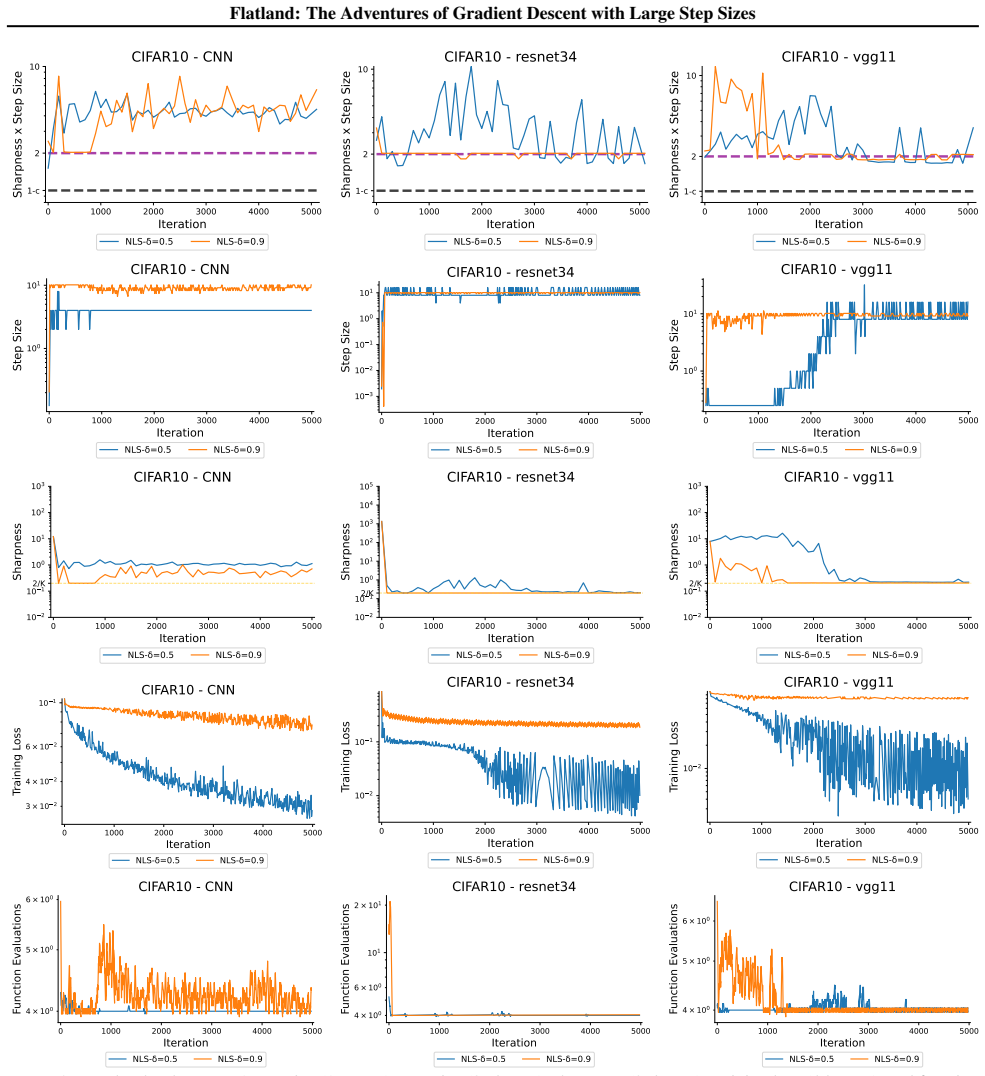
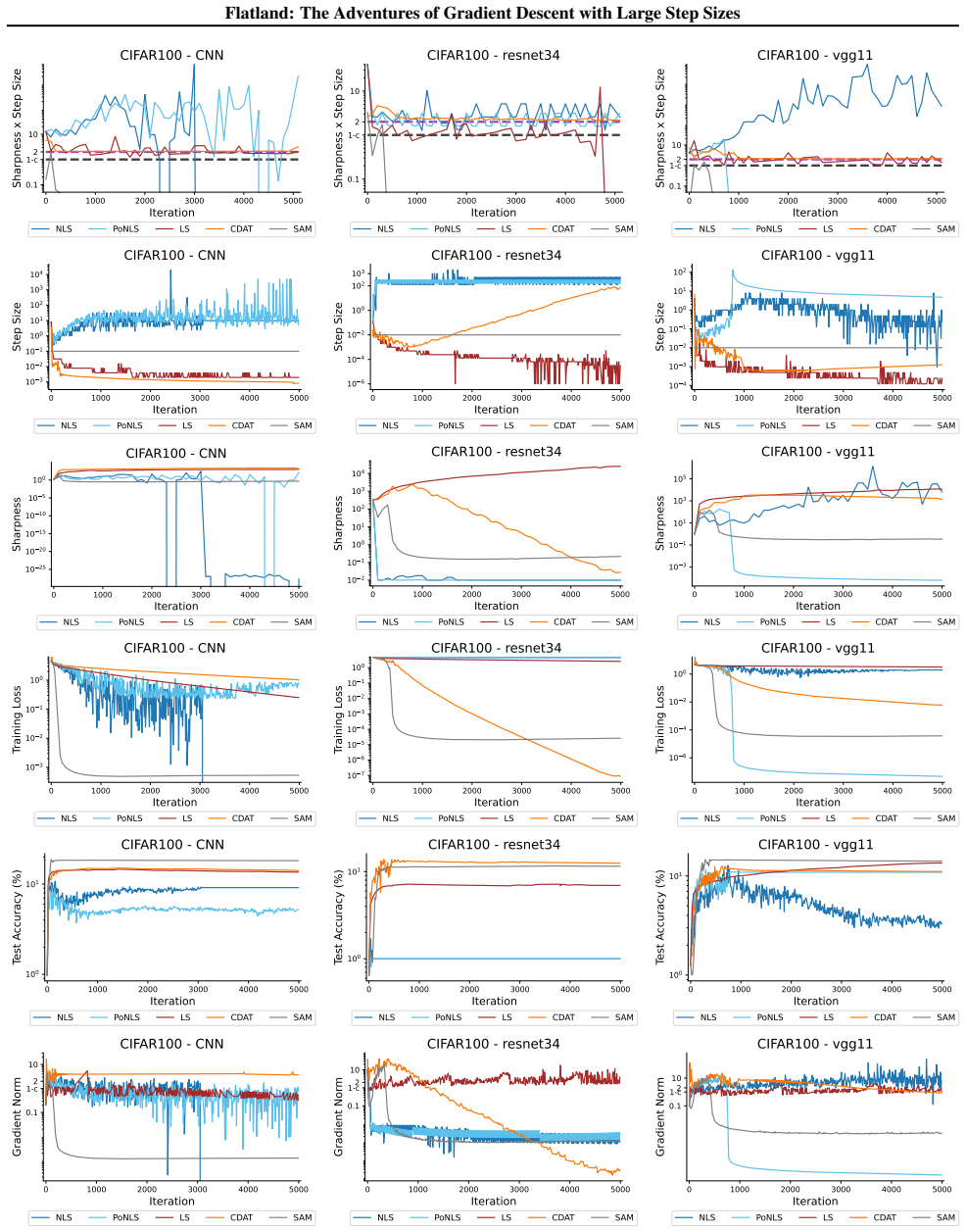
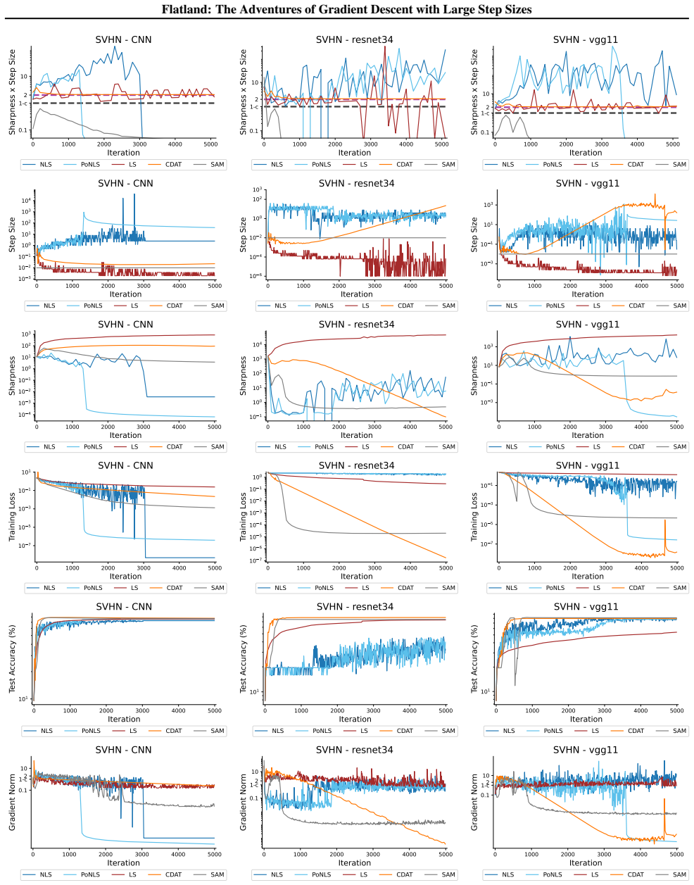
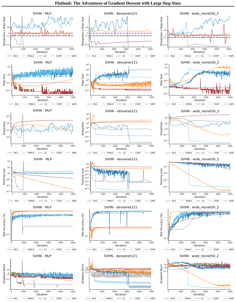
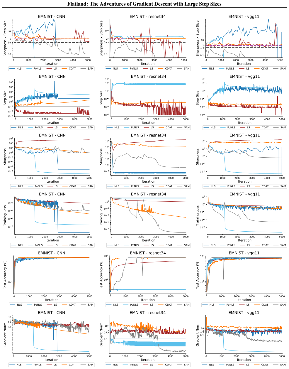
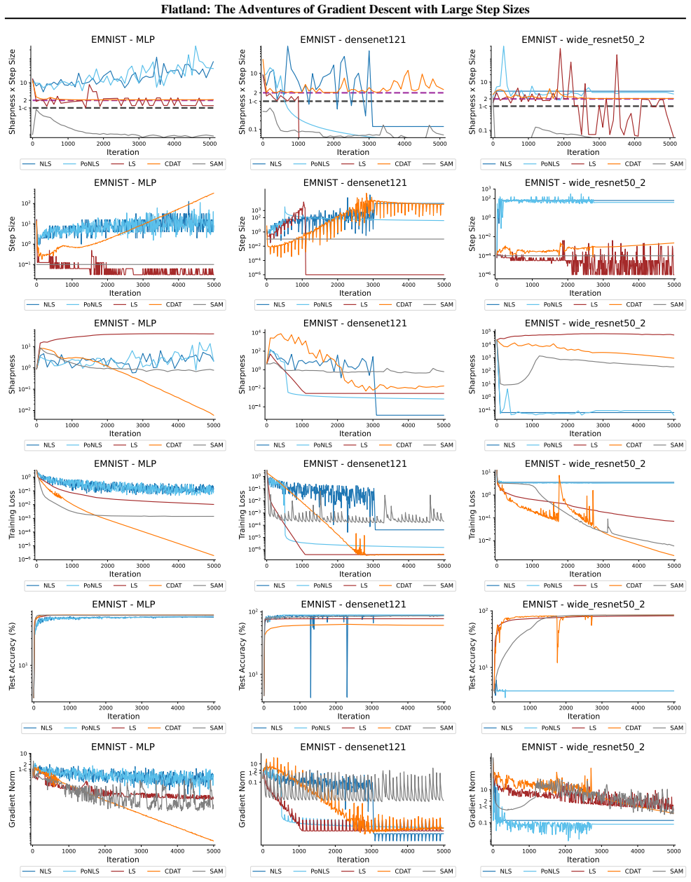
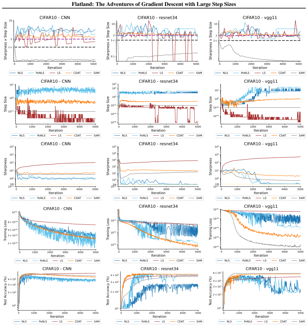
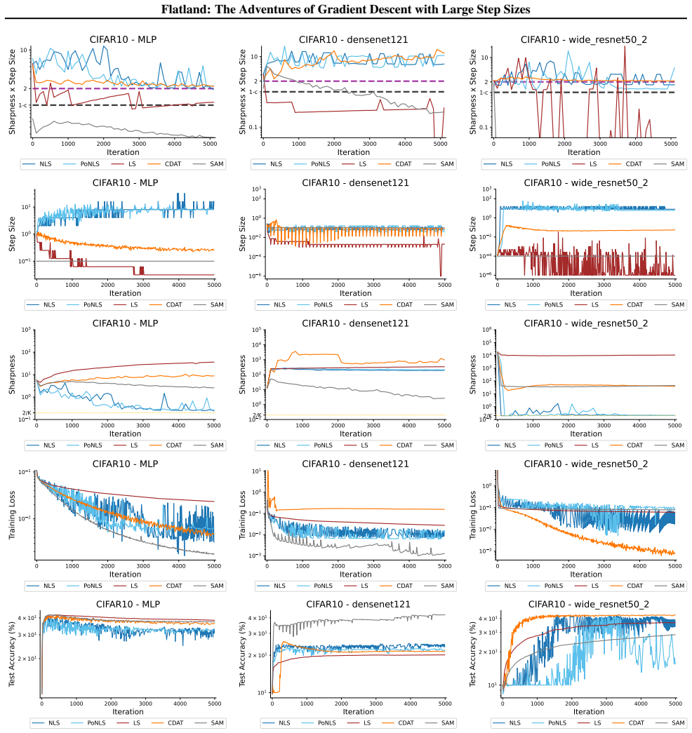
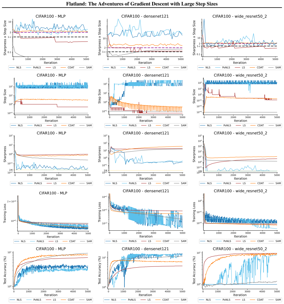
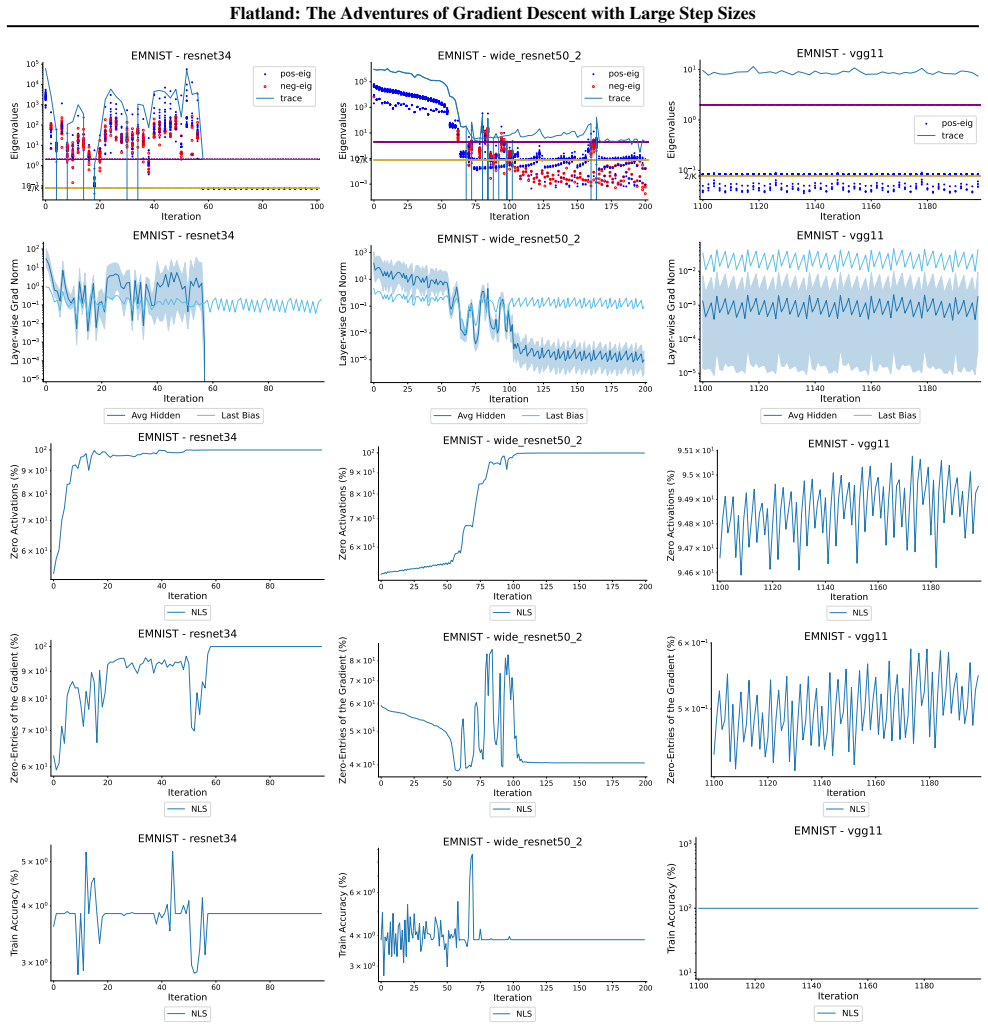
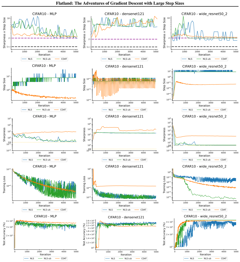
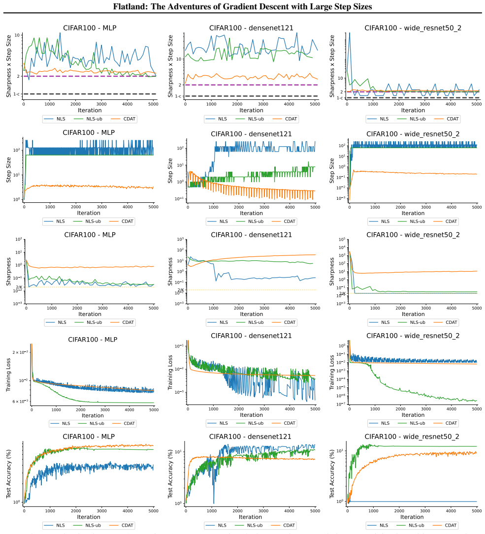
First-order adaptive methods can be designed to provably produce large step sizes under local gradient continuity and operate at the edge of stability throughout training, with the loss decreasing nonmonotonically and the step size-sharpness product staying above 2. These methods can minimize sharpness to its global minimum. Avoiding globally flat regions early in training prevents slower convergence and poorer generalization, while self-stabilization allows gradient descent to enter slightly sharper valleys successfully.
What carries the argument
The edge of stability condition, defined as the step size multiplied by the largest Hessian eigenvalue exceeding 2, which the adaptive methods maintain using local continuity to permit large steps.
Load-bearing premise
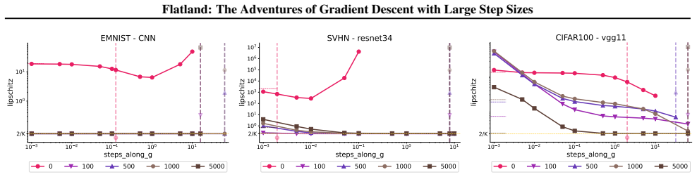
The objective function's gradient is locally Lipschitz continuous or Hölder continuous, rather than requiring global L-smoothness.
What would settle it
A counterexample where an adaptive method with large step sizes fails to keep the step size-sharpness product above 2 while still achieving faster convergence than standard gradient descent with small steps.
Figures


read the original abstract
The training of neural networks often entails objective functions that are not globally $L$-smooth. For these functions, it is both theoretically and practically difficult to reply to the question: what is the largest possible step size that ensures the convergence of gradient descent (GD)? We address this longstanding open question in deep learning by providing a unifying definition of "large" step sizes that requires only local Lipschitz (or even H\"older) continuity of the gradient. We design first-order adaptive methods that provably yield large step sizes and show that they operate at the edge of stability (EoS) right from the start of the training. In particular, the loss decreases nonmonotonically and the product between the step size and sharpness, i.e., the largest eigenvalue of the Hessian, stays above the EoS threshold of 2 throughout training. Using our method, we are also able to minimize the sharpness all the way down to its global minimum. Contrary to expectation, we find that encountering globally-flat regions too early in the training may both slow down convergence and jeopardize the generalization ability of the network. Exploiting a self-stabilization argument, we allow GD to enter slightly sharper valleys and turn unsuccessful training runs into very successful ones.
Editorial analysis
A structured set of objections, weighed in public.
Referee Report
Summary. The paper defines 'large' step sizes for gradient descent using only local Lipschitz or Hölder continuity of the gradient (instead of global L-smoothness). It introduces first-order adaptive methods that provably achieve such steps and operate at the edge of stability (EoS) from the first iteration onward, characterized by non-monotonic loss decrease and step-size × sharpness remaining above the threshold of 2. The work also shows how to drive sharpness to its global minimum and uses a self-stabilization argument to allow entry into slightly sharper regions, converting failed runs into successful ones.
Significance. If the local-continuity framework and the EoS guarantees hold, the results supply a principled way to select and adapt large steps in the non-globally-smooth regimes typical of deep learning, directly linking theory to the observed edge-of-stability phenomenon. The self-stabilization mechanism and the empirical demonstration that early global flatness can harm generalization are noteworthy contributions.
major comments (2)
- [§3.2, Theorem 2] §3.2 and Theorem 2: the proof that the adaptive methods keep step-size × sharpness ≥ 2 from iteration 1 onward invokes only local Lipschitz/Hölder continuity; the argument appears to require an implicit uniformity condition on how the local constant evolves relative to the chosen step size, which is not guaranteed by the stated assumption alone and is load-bearing for the 'provably operate at EoS right from the start' claim.
- [§5.1] §5.1, the self-stabilization construction: the claim that GD can be steered into slightly sharper valleys without instability rests on the same local-continuity premise; an explicit bound relating the local constant to the step-size adaptation is needed to make the 'turn unsuccessful training runs into successful ones' result rigorous.
minor comments (2)
- [§2] Notation for the local Hölder exponent and the adaptive step-size rule should be introduced once in §2 and used consistently thereafter.
- [Figure 4] Figure 4 caption should explicitly state the number of independent runs and the precise definition of 'sharpness' used in the plot.
Simulated Author's Rebuttal
We thank the referee for the careful reading and constructive feedback. We address the two major comments point by point below, indicating planned revisions where they strengthen the rigor of the claims.
read point-by-point responses
-
Referee: [§3.2, Theorem 2] §3.2 and Theorem 2: the proof that the adaptive methods keep step-size × sharpness ≥ 2 from iteration 1 onward invokes only local Lipschitz/Hölder continuity; the argument appears to require an implicit uniformity condition on how the local constant evolves relative to the chosen step size, which is not guaranteed by the stated assumption alone and is load-bearing for the 'provably operate at EoS right from the start' claim.
Authors: We appreciate the referee identifying this point. The adaptive methods select the step size at each iterate using only local first-order information (gradient and a local sharpness estimate) at the current point, so the local Lipschitz/Hölder assumption is applied pointwise. The one-step analysis in Theorem 2 then shows that the chosen step size satisfies step-size × sharpness ≥ 2 by construction. Nevertheless, to eliminate any ambiguity about the evolution of the local constant, we will add a short clarifying lemma in §3.2 that explicitly bounds the change in the local constant over a single step under the adaptive rule. revision: yes
-
Referee: [§5.1] §5.1, the self-stabilization construction: the claim that GD can be steered into slightly sharper valleys without instability rests on the same local-continuity premise; an explicit bound relating the local constant to the step-size adaptation is needed to make the 'turn unsuccessful training runs into successful ones' result rigorous.
Authors: We agree that an explicit bound would make the self-stabilization argument fully rigorous. In the revised version we will insert, in §5.1, a bound that relates the local continuity constant to the adaptive step-size choice, thereby justifying that the method can enter slightly sharper regions without instability and convert unsuccessful runs into successful ones. revision: yes
Circularity Check
No circularity: definition and claims are independent of fitted inputs or self-referential reductions
full rationale
The paper defines 'large' step sizes via local Lipschitz/Hölder continuity of the gradient—an external modeling choice stated upfront—and then constructs adaptive first-order methods whose properties (non-monotonic loss decrease, stepsize × sharpness ≥ 2 from iteration 1) are derived as consequences rather than presupposed. No equation or claim reduces a prediction to a fitted parameter by construction, no uniqueness theorem is imported from prior self-work, and the self-stabilization argument is presented as an exploitation of the local-continuity setting rather than an input. The derivation chain therefore remains self-contained against external benchmarks and does not match any of the enumerated circularity patterns.
Axiom & Free-Parameter Ledger
axioms (1)
- domain assumption The gradient of the objective is locally Lipschitz continuous or Hölder continuous.
Reference graph
Works this paper leans on
-
[1]
Notice that the compactness of the L0 level set is implied by the coercivity of the function f, i.e., lim ||w||→∞ f(w) =∞
As∇fis continuous, it is uniformly continuous on the compact set, hence lim i→∞ ∥∇f(z ki)− ∇f(w ki)∥= 0, which by (27) gives the convergence to zero of the subsequence of the gradient. Notice that the compactness of the L0 level set is implied by the coercivity of the function f, i.e., lim ||w||→∞ f(w) =∞ . This property holds for MSE loss functions appli...
2025
-
[2]
23 Flatland: The Adventures of Gradient Descent with Large Step Sizes
The mean squared error (MSE)-loss:l:R n →R,l(w) = 1 Km Pm i=1 ∥n(w, xi)−y i∥2 2. 23 Flatland: The Adventures of Gradient Descent with Large Step Sizes
-
[3]
Lemma B.23.Let (x,ˆy)be a data point, f the MSE-loss for the output of the network nx :R n →R K with identity afterwards
The cross-entropy loss:l:R n →R,l(w) = 1 m Pm i=1 PC k=1 −yi,k log(n(w, xi)k). Lemma B.23.Let (x,ˆy)be a data point, f the MSE-loss for the output of the network nx :R n →R K with identity afterwards. Assume that the last layer is linear, i.e. nx(w) =W x ′(w′) +b , where x′(w′) is the output of the previous layer and denote byw ′ :=w\{W, b}all parameters ...
-
[4]
the weights of the last layer has the form ∇2 W f(w) = 2 K IK ⊗x ′x′T ,∇ 2 bf(w) = 2 K IK,∇ 2 W,bf(w) = 2 K IK ⊗x ′
The subhessian of w.r.t. the weights of the last layer has the form ∇2 W f(w) = 2 K IK ⊗x ′x′T ,∇ 2 bf(w) = 2 K IK,∇ 2 W,bf(w) = 2 K IK ⊗x ′
-
[5]
The trace of the subhessian is given by trace(∇ 2 (W,b)f(w)) = 2(∥x ′∥2 + 1)
-
[6]
The biggest eigenvalue of the hessian is at least 2 K , i.e.λ 1(∇2 wf(w))≥ 2 K . Proof.We start with some general derivations for our loss functional: f(w) = 1 K ∥nx(w)−ˆy∥2 2,∇ wf(w) = 2 K KX i=1 (nx,i(w)−ˆyi)∇nx,i(w) ∇2f(w) = 2 K KX i=1 ∇wnx,i(w)∇wnx,i(w)T + (nx,i(w)−ˆyi)∇2 wnx,i(w)
-
[7]
Letw i denote the rows ofW, then ∇wj nx,i(w) =δ i,jx′,∇ bj nx,i(w) =δ i,j,∇ 2 W nx,i(w) =∇ 2 bnx,i(w) =∇ 2 W,bnx,i = 0, ⇒ ∇ 2 W f(w) = 2 K x′x′T 0
As we are interested in the last layer ofn x, which is given byW x ′ +b. Letw i denote the rows ofW, then ∇wj nx,i(w) =δ i,jx′,∇ bj nx,i(w) =δ i,j,∇ 2 W nx,i(w) =∇ 2 bnx,i(w) =∇ 2 W,bnx,i = 0, ⇒ ∇ 2 W f(w) = 2 K x′x′T 0. . .0 0x ′x′T . . .0 . . . . . . . . . . . . 0 0. . . x ′x′T ,∇ 2 bf(w) = 2 K KX i=1 eieT i ,∇ W,bf(w) = 2 K x′ 0. . .0...
-
[8]
With this at hand, it is straightforward to calculate the trace trace(∇2 (W,b)f(w)) = 2 K KX i=1 ∥∇(W,b)nx,i(w)∥2 = 2 K KX i=1 ∥x∥2 + 1 = 2(∥x∥2 + 1)
-
[9]
Which we use with the sub-block∇ 2 bf(w)which has eigenvalues 2 K , as calculated previously
This can be seen by Cauchy’s interlacing theorem (Horn & Johnson, 2012), which implies for a symmetric matrix A= B C C T D, , λ 1(A)≥λ 1(D). Which we use with the sub-block∇ 2 bf(w)which has eigenvalues 2 K , as calculated previously. As the previous Lemma was just for a single data point by the linearity of the loss function we can easily derive a result...
2012
-
[10]
Therefore, again trace ∇2 (W,b)f(w) = 2 1 m Pm i=1 ∥x′ i∥2 2 + 1 and the biggest eigenvalue of the Hessian w.r.t
The subhessian is given by ∇2 W f(w) = 2 K IK ⊗ 1 m mX i=1 x′ ix′T i ,∇ 2 bf(w) = 2 K IK,∇ W,bf(w) = 2 K IK ⊗ 1 m mX i=1 x′. Therefore, again trace ∇2 (W,b)f(w) = 2 1 m Pm i=1 ∥x′ i∥2 2 + 1 and the biggest eigenvalue of the Hessian w.r.t. the whole data set is lower bounded by 2 K . 24 Flatland: The Adventures of Gradient Descent with Large Step Sizes Pro...
-
[11]
the weights of the last layer has the form ∇2 W f(w) = diag(p)−pp T ⊗x ′x′T ,∇ 2 bf(w) = diag(p)−pp T ,∇ 2 W,bf(w) = diag(p)−pp T ⊗x ′
The subhessian of w.r.t. the weights of the last layer has the form ∇2 W f(w) = diag(p)−pp T ⊗x ′x′T ,∇ 2 bf(w) = diag(p)−pp T ,∇ 2 W,bf(w) = diag(p)−pp T ⊗x ′
-
[12]
instantaneous
The trace of the subhessian is given by trace(∇ 2 (W,b)f(w)) = 1− ∥p∥ 2 2 (1 +∥x ′∥2 2). Proof. As ˆyis a one-hot encoding ˆy=e k for one k∈ {1, . . . , K} , the loss function of the network and its gradient can thus be written as f(w) =−n x(w)k + log KX j=1 en(w)j , ∇wf(w) =−∇ wnx,k(w) + KX j=1 pj∇wnx,j(w), ∇2 wf(w) =−∇ 2 wnx,k(w) + KX j=1 pl ∇wn...
2009
discussion (0)
Sign in with ORCID, Apple, or X to comment. Anyone can read and Pith papers without signing in.