REVIEW 3 major objections 6 minor 1 cited by
Estimate Sonic Mach Number in the Interstellar Medium with Convolutional Neural Network
T0 review · 3 major / 6 minor · reviewed 2026-08-12 · deepseek-v4-flash
Pith's one-line read A convolutional neural network can estimate the sonic Mach number of interstellar gas directly from spectroscopic maps.
desk verdict First CNN for sonic Mach number is an incremental but sound proof-of-concept; the abstract's generalization claim outruns the retrain-per-condition experiments. read the letter →
The pith
A machine-rendered reading of the paper's core claim, the machinery that carries it, and where it could break.
The reading
What carries the argument
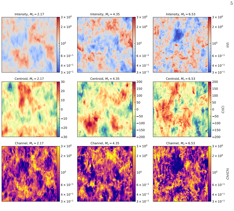
The load-bearing mechanism is the morphological encoding of $M_s$ in projected maps, captured by a CNN. The paper identifies the physical correlation as the growth of small-scale density fluctuations and filamentary structures when $M_s$ increases, driven by shocks; intensity maps carry this most directly, while velocity centroids mix in intensity-weighted velocity information and thin velocity channels are dominated by velocity caustics, which makes them less sensitive to $M_s$ but more useful for 3D mapping. The CNN architecture, with convolution, pooling, batch normalization, and fully connected layers, learns the mapping from 32x32-cell map patches to a scalar $M_s$ prediction using mean-squared-error training on roughly 0.6 million subfields per iteration.
What would settle it
Compare CNN predictions, trained only on idealized isothermal solenoidally driven simulations, against independently measured sonic Mach numbers in real molecular clouds (for example, from column-density PDF widths or from Zeeman-inferred fields combined with velocity dispersions), and check whether the median absolute error stays within the claimed 0.5 to 1.5 range; a second test is to run the network on a simulation that includes radiative transfer and self-gravity and measure the error increase.
Extended reading notes
Core claim
The central claim is that the spatial pattern of gas emission encodes the sonic Mach number, and a CNN can decode it. Using six $512^{3}$ isothermal ideal-MHD simulations with similar Alfvénic Mach number but sonic Mach numbers from 2.17 to 11.02, the authors generate synthetic position-position-velocity cubes, cut them into 32x32-cell subfields, and train a CNN to predict the local $M_s^{\rm sub}$ defined by the line-of-sight velocity dispersion in each subfield. The network learns that higher $M_s$ produces more small-scale, shock-dominated filamentary structures in intensity and centroid maps, and it transfers this association across different magnetic field strengths, inclinations, noise levels, and missing low spatial frequencies. The paper reports median absolute errors around 0.5 in the noise-free perpendicular-field case, generally below 2 even at 100% noise, and below 1 when low spatial frequencies are removed, supporting the claim that the morphologies are robustly correlated with $M_s$.
Load-bearing premise
The model's predictive power depends on the simulated MHD maps being representative of real spectroscopic observations, since the network learns only morphologies that appear in the six idealized isothermal, solenoidally driven simulations used for training.
Editorial extensions
If this is right
- Combined with CNN-estimated $M_A$, the predicted $M_s$ yields magnetic field strength through $B = c_s\sqrt{4\pi\rho}M_s M_A^{-1}$, enabling magnetic-field mapping in molecular clouds.
- Using thin velocity channel maps rather than intensity maps makes it possible to predict the 3D distribution of $M_s$, which is needed for 3D Galactic magnetic field reconstruction when combined with the rotation curve.
- The network remains accurate when low spatial frequencies are removed (median errors below 1 for filters out to wavenumber 30), so it can be applied to interferometric observations with missing short baselines.
- Adding Gaussian noise up to a noise ratio of 100% keeps median errors below about 2, and intensity maps remain the most accurate input type across noise levels.
Reading between the lines
- If the morphology-to-$M_s$ mapping generalizes, the same CNN architecture could be retrained to output $M_s$ and $M_A$ simultaneously from one set of maps, giving a direct pixel-by-pixel estimate of the compressibility parameter $\beta = 2(M_A/M_s)^2$.
- A natural test of the paper's hidden assumption is to train on the idealized isothermal simulations and then evaluate on simulations that include radiative transfer, self-gravity, and outflow feedback; the Appendix's unseen-data result suggests the error increase would be measurable and would indicate when retraining is needed.
- A practical consequence for surveys: the reported median errors of 0.5 to 1.5 imply the method can reliably separate subsonic, transonic, and supersonic regions, but may not resolve fine differences in $M_s$ for precision turbulence studies.
Signed reviews
Editorial analysis
A structured set of objections, weighed in public.
Referee Report
Summary. The paper trains a convolutional neural network on 32x32 subfields drawn from six isothermal, solenoidally driven MHD turbulence simulations, using integrated intensity, velocity centroid, and velocity channel maps as inputs to predict the sonic Mach number Ms. The target label is a local Ms defined through the line-of-sight velocity dispersion of each subfield. The authors report median absolute errors of roughly 0.5-2 across different Ms, magnetic field inclination angles, added Gaussian noise levels, and removal of low spatial frequencies, and conclude that the CNN can predict Ms under a variety of observational conditions. An appendix tests one additional simulation not used in training and reports that prediction errors increase for that unseen simulation.
Significance. If the generalization claim held, this would be a practically useful tool: it would allow spatially resolved Ms estimates from spectroscopic maps without region-by-region PDF fitting, and channel-map predictions could in principle support 3D magnetic field strength measurements. The paper is also a useful proof of concept for applying CNNs to synthetic PPV observations, and it explicitly compares three commonly used map types. However, the quantitative evidence in the main text comes from subfields of the same six simulations used for training, and each robustness experiment retrains a new model for the condition being tested. The single out-of-distribution test in Appendix B shows degraded performance. The central claim is therefore not yet supported at the level stated in the abstract; additional fixed-network or leave-one-out evaluations are needed.
major comments (3)
- [Abstract; Sections 3.3-3.5] The abstract claims that the CNN can predict Ms 'under various conditions, including different magnetic fields and levels of observational noise,' but the experiments in Sections 3.3-3.5 retrain the network separately for each condition: Section 3.3 states that the simulation boxes are rotated 'and retrain the CNN model accordingly,' Section 3.4 says the model 'is trained to make predictions' at each noise level, and Section 3.5 applies the k-space filter 'before CNN training.' Figures 5-7 therefore measure how well a freshly fitted model performs on data drawn from the same distribution as its training set, not whether a single trained model transfers across conditions. Real observations will have unknown combinations of inclination, noise, and spatial filtering, so the paper should include a fixed-network evaluation across a parameter sweep, or at minimum a leave-one-condition-out test, before claiming robustness under varied conditions.
- [Section 3.2 and Appendix B] The main demonstration of predictive accuracy, including Figure 3 and Figure 4, uses simulation min06 (Ms = 11.02), which Appendix B explicitly identifies as included in the training process. The headline error statistics are therefore in-sample or near-in-sample. The only genuinely held-out test, Appendix B's simulation min07 (Ms = 10.50, MA = 0.81), shows increased prediction error, but the manuscript reports this only as qualitative histograms without quoting the median and quartile errors for seen versus unseen data. Please quantify the degradation for each map type and present this as a central robustness metric rather than a deferred appendix result.
- [Section 2.4, Eq. (4)] The training label M_sub_s is defined using the line-of-sight velocity dispersion v_sub in each 32x32 subfield. The paper does not justify that this is an unbiased proxy for the true local sonic Mach number of the subfield. Along a given LOS, the observed velocity dispersion mixes turbulent velocity fluctuations with projection and density-weighting effects, and the relation between v_sub and the actual 3D velocity dispersion may vary with Ms and with magnetic field geometry. Since the label itself is constructed from the same PPV data that provide the input maps, the measured prediction errors partly reflect the correlation between the label and the local statistics of the input rather than an independent physical quantity. Please add a validation against the true 3D velocity dispersion or another independently defined Ms for the subfields, and report the resulting bias.
minor comments (6)
- [Section 3.4, first paragraph] The text says 'Fig. 5 presents the absolute error' for the noise analysis, but the figure shown for noise is Figure 6; Figure 5 is the inclination-angle figure. Please correct the cross-reference.
- [Abstract and Section 3.4] The abstract states that the median uncertainty ranges from 0.5 to 1.5, while Section 3.4 reports median errors rising to approximately 2-2.25 in the highest noise cases. These numbers should be reconciled or the abstract should be qualified by noise level.
- [Section 3.5] The removed spatial frequency ranges '0 - 10, 0 - 20, and 0 - 30' are not defined in physical units; please state the normalization of k (for example, k in units of 2π/L_box) and, for the interferometric motivation, explain how these cutoffs map to baseline coverage.
- [Section 2.3 and Figure 1] The architecture description lacks quantitative details: the number and size of convolution kernels, pooling sizes, number of fully connected units, activation functions, optimizer, learning rate, batch size, and the exact training/validation split are not stated. These details are needed to reproduce the results and to assess possible overfitting.
- [Section 2.5] The description of random rotation is ambiguous: it should state whether rotations are restricted to multiples of 90 degrees or are arbitrary angles, since arbitrary rotations require interpolation and effectively change the pixel statistics.
- [Table 1] There is a formatting error in the caption ('T able 1'), and the superscript/subscript notation for M_sub_s should be made consistent throughout the text and figures.
Circularity Check
Main-text 'predictions' are in-sample or per-condition refits; the only held-out test (Appendix B) shows degraded accuracy, so the robustness claim is partly an artifact of the training protocol.
-
fitted input called prediction
[Section 2.5; Section 3.2; Table 1; Appendix B]
"the original non-rotated datasets can be used as validation and a method of creating prediction test scenarios."
The 'prediction test scenarios' are drawn from the same six simulations (Table 1) that supplied the ~0.6 million training subfields; Section 3.2 evaluates on simulation Ms = 11.02 (min06 in Table 1) without a held-out split. The only explicitly unseen simulation, min07 in Appendix B, is reported to have increased error. The headline median uncertainties (0.5-1.5) are therefore in-sample fit residuals, not out-of-sample prediction errors, so calling them 'CNN-predicted Ms' overstates what was measured.
-
fitted input called prediction
[Section 3.3, Fig. 5]
"we rotate the simulation boxes to achieve four different inclination angles (90, 60, 30, and 0 degrees), generate synthetic spectroscopic data, and retrain the CNN model accordingly."
A separate CNN is fitted for each inclination angle, and the box-plot errors in Fig. 5 are computed on data from that same inclination. The experiment thus measures how well each condition-specific fit matches its own training condition, not how a single network trained on one geometry transfers to other magnetic-field orientations. The abstract's claim of prediction 'under various conditions, including different magnetic fields' is not established by this protocol.
1 more flagged steps
-
fitted input called prediction
[Section 3.4 and 3.5, Figs. 6-7]
"This analysis is conducted for three types of input maps—intensity, centroid, and channel maps, all with an inclination angle of 90 degrees—on which the CNN model is trained to make predictions."
For each noise ratio the model is retrained on that noise level, and in Section 3.5 the k-space filter is applied 'before CNN training,' so each reported error is a per-condition training residual. The claimed robustness to noise and missing low spatial frequencies is therefore a property of refitting a model to each condition, not of a single predictive model transferred across conditions.
full rationale
No circularity is found in the physical derivation: the CNN is a supervised regressor from synthetic spectroscopic maps to a locally defined M_sub^s, and no load-bearing argument reduces to a self-citation or to a definitional identity. The circularity is in the evaluation protocol. The main-text accuracy figures are in-sample (same six simulations used for training, with augmentation) or per-condition refits (Sections 3.3-3.5), so the errors reported are fit residuals rather than predictions. The paper itself supplies the decisive control: Appendix B tests a genuinely unseen simulation (min07) and reports that prediction error increases, which confirms that the earlier numbers were not out-of-sample. This is why the score is 6 rather than higher; the appendix prevents the claim from being entirely tautological. The simulation-realism concerns (radiative transfer, gravity, feedback deferred in Section 4.1) are generalization risks, not circularity, and are not scored here.
Assumptions & free parameters
free parameters (5)
- CNN weights (trainable parameters) =
learned from ~0.6 million subfields per training iteration
- CNN architecture hyperparameters =
not reported (e.g., optimizer, learning rate, kernel counts)
- Input map normalization =
normalized by maximum map value
- Channel width Delta v =
chosen such that Delta v < sqrt(delta v^2); exact value not stated
- Training set size and iterations =
~0.6 million subfields per iteration; at least 20 iterations
assumptions (3)
- domain assumption ZEUS-MP/3D isothermal, solenoidally driven ideal MHD simulations represent the density and velocity structure of the ISM.
- domain assumption The local line-of-sight velocity dispersion in a 32x32 subfield is an adequate proxy for the sonic Mach number of that subfield.
- domain assumption Morphological features in intensity, centroid, and channel maps are sufficiently determined by Ms that a CNN can learn a mapping that generalizes across magnetic field strengths, noise, and missing spatial frequencies.
Cite this review
Pith. "Pith review of Estimate Sonic Mach Number in the Interstellar Medium with Convolutional Neural Network." pith.science (2026). https://pith.science/paper/DQ4W34JT
@misc{pith2026241111157,
  author       = {Pith},
  title        = {Pith review of: Estimate Sonic Mach Number in the Interstellar Medium with Convolutional Neural Network},
  year         = {2026},
  howpublished = {\url{https://pith.science/paper/DQ4W34JT}},
  note         = {Machine review of arXiv:2411.11157}
}
abstract
Understanding the role of turbulence in shaping the interstellar medium (ISM) is crucial for studying star formation, molecular cloud evolution, and cosmic ray propagation. Central to this is the measurement of the sonic Mach number ($M_s$), which quantifies the ratio of turbulent velocity to the sound speed. In this work, we introduce a convolutional neural network (CNN)-based approach for estimating $M_s$ directly from spectroscopic observations. The approach leverages the physical correlation between increasing $M_s$ and the shock-induced small-scale fluctuations that alter the morphological features in intensity, velocity centroid, and velocity channel maps. These maps, derived from 3D magnetohydrodynamic (MHD) turbulence simulations, serve as inputs for the CNN training. By learning the relationship between these structural features and the underlying turbulence properties, CNN can predict $M_s$ under various conditions, including different magnetic fields and levels of observational noise. The median uncertainty of the CNN-predicted $M_s$ ranges from 0.5 to 1.5 depending on the noise level. While intensity maps offer lower uncertainty, channel maps have the advantage of predicting the 3D $M_s$ distribution, which is crucial in estimating 3D magnetic field strength. Our results demonstrate that machine-learning-based tools can effectively characterize complex turbulence properties in the ISM.
Figures


Figures from the paper (6 more)


Forward citations
Cited by 1 Pith paper
-
Characterizing 3D Magnetic Fields and Turbulence in H I Clouds
A neural network maps H I spectral cubes to 3D magnetic field orientation, strength, sonic and Alfven Mach numbers, and it is applied to two FAST-survey clouds in Monoceros.
Reference graph
Works this paper leans on
-
[1]
2015, TensorFlow: Large-Scale Machine Learning on Heterogeneous Systems
Abadi, M., Agarwal, A., Barham, P., et al. 2015, TensorFlow: Large-Scale Machine Learning on Heterogeneous Systems. https://www.tensorflow.org/
2015
-
[2]
Armstrong, J. W., Rickett, B. J., & Spangler, S. R. 1995, ApJ, 443, 209, doi: 10.1086/175515
doi:10.1086/175515 1995
-
[3]
2011, MNRAS, 416, 1436, doi: 10.1111/j.1365-2966.2011.19141.x
Ballesteros-Paredes, J., V´ azquez-Semadeni, E., Gazol, A., et al. 2011, MNRAS, 416, 1436, doi: 10.1111/j.1365-2966.2011.19141.x
arXiv 2011
-
[4]
Beattie, J. R., & Federrath, C. 2019, Monthly Notices of the Royal Astronomical Society, 492, 668, doi: 10.1093/mnras/stz3377
-
[5]
Beattie, J. R., Krumholz, M. R., Federrath, C., Sampson, M. L., & Crocker, R. M. 2022, Frontiers in Astronomy and Space Sciences, 9, doi: 10.3389/fspas.2022.900900
-
[6]
2005, ApJL, 624, L93, doi: 10.1086/430702
Beresnyak, A., Lazarian, A., & Cho, J. 2005, ApJL, 624, L93, doi: 10.1086/430702
doi:10.1086/430702 2005
-
[7]
Berkhuijsen, E. M., & Fletcher, A. 2008, Monthly Notices of the Royal Astronomical Society: Letters, 390, L19, doi: 10.1111/j.1745-3933.2008.00526.x
arXiv 2008
-
[8]
2019, Astronomy & Astrophysics, 632, A17, doi: 10.1051/0004-6361/201935951
Bracco, A., Ghosh, T., Boulanger, F., & Aumont, J. 2019, Astronomy & Astrophysics, 632, A17, doi: 10.1051/0004-6361/201935951
Show all 77 references
-
[9]
Brunt, C. M. 2010, A&A, 513, A67, doi: 10.1051/0004-6361/200913506
2010 doi
-
[10]
2018, ApJ, 863, 118, doi: 10.3847/1538-4357/aad002
Burkhart, B. 2018, ApJ, 863, 118, doi: 10.3847/1538-4357/aad002
2018 doi
-
[11]
2012, The Astrophysical Journal Letters, 755, L19, doi: 10.1088/2041-8205/755/1/L19
Burkhart, B., & Lazarian, A. 2012, The Astrophysical Journal Letters, 755, L19, doi: 10.1088/2041-8205/755/1/L19
2012 doi
-
[12]
2009, The Astrophysical Journal, 708, 1204, doi: 10.1088/0004-637X/708/2/1204
Burkhart, B., Stanimirovi´ c, S., Lazarian, A., & Kowal, G. 2009, The Astrophysical Journal, 708, 1204, doi: 10.1088/0004-637X/708/2/1204
2009 doi
-
[13]
2010, ApJ, 710, 853
Chepurnov, A., & Lazarian, A. 2010, ApJ, 710, 853
2010
-
[14]
Crutcher, R. M. 2004, in The Magnetized Interstellar Medium, ed. B. Uyaniker, W. Reich, & R. Wielebinski, 123–132
2004
-
[15]
Crutcher, R. M. 2012, ARA&A, 50, 29, doi: 10.1146/annurev-astro-081811-125514
2012 doi
-
[16]
Elmegreen, B. G. 1993, ApJL, 419, L29, doi: 10.1086/187129
1993 doi
-
[17]
2010, The Astrophysical Journal, 710, 125, doi: 10.1088/0004-637X/710/1/125
Esquivel, A., & Lazarian, A. 2010, The Astrophysical Journal, 710, 125, doi: 10.1088/0004-637X/710/1/125
2010 doi
-
[18]
2015, MNRAS, 448, 3297, doi: 10.1093/mnras/stv180
Federrath, C., & Banerjee, S. 2015, MNRAS, 448, 3297, doi: 10.1093/mnras/stv180
2015 doi
-
[19]
Federrath, C., & Klessen, R. S. 2012, ApJ, 761, 156, doi: 10.1088/0004-637X/761/2/156
2012 doi
-
[20]
S., & Schmidt, W
Federrath, C., Klessen, R. S., & Schmidt, W. 2008, ApJL, 688, L79, doi: 10.1086/595280 16
2008 doi
-
[21]
C., Ruffolo, D., Chuychai, P., et al
Ghilea, M. C., Ruffolo, D., Chuychai, P., et al. 2011, ApJ, 741, 16, doi: 10.1088/0004-637X/741/1/16
2011 doi
-
[22]
1995, ApJ, 438, 763, doi: 10.1086/175121
Goldreich, P., & Sridhar, S. 1995, ApJ, 438, 763, doi: 10.1086/175121
1995 doi
-
[23]
2022, ApJ, 934, 7, doi: 10.3847/1538-4357/ac76bf
Ha, T., Li, Y., Kounkel, M., et al. 2022, ApJ, 934, 7, doi: 10.3847/1538-4357/ac76bf
2022 doi
-
[24]
C., Norman, M
Hayes, J. C., Norman, M. L., Fiedler, R. A., et al. 2006, The Astrophysical Journal Supplement Series, 165, 188, doi: 10.1086/504594
2006 doi
-
[25]
S., Benjamin, R
Hill, A. S., Benjamin, R. A., Kowal, G., et al. 2008, The Astrophysical Journal, 686, 363, doi: 10.1086/590543
2008 doi
-
[26]
Hu, Y., Federrath, C., Xu, S., & Mathew, S. S. 2022, MNRAS, 513, 2100, doi: 10.1093/mnras/stac972
2022 doi
-
[27]
2023, Monthly Notices of the Royal Astronomical Society, 524, 2379–2394, doi: 10.1093/mnras/stad1996
Hu, Y., & Lazarian, A. 2023, Monthly Notices of the Royal Astronomical Society, 524, 2379–2394, doi: 10.1093/mnras/stad1996
2023 doi
- [28]
-
[29]
Hu, Y., Lazarian, A., Alina, D., Pogosyan, D., & Ho, K. W. 2023, MNRAS, 524, 2994, doi: 10.1093/mnras/stad1924
2023 doi
-
[30]
2022, The Astrophysical Journal, 941, 92, doi: 10.3847/1538-4357/ac9df0
Hu, Y., Lazarian, A., Beck, R., & Xu, S. 2022, The Astrophysical Journal, 941, 92, doi: 10.3847/1538-4357/ac9df0
2022 doi
-
[31]
2020, ApJ, 905, 129, doi: 10.3847/1538-4357/abc3c6
Hu, Y., Lazarian, A., & Bialy, S. 2020, ApJ, 905, 129, doi: 10.3847/1538-4357/abc3c6
2020 doi
-
[32]
2021, The Astrophysical Journal, 912, 2, doi: 10.3847/1538-4357/abedb7
Hu, Y., Lazarian, A., & Stanimirovi´ c, S. 2021, The Astrophysical Journal, 912, 2, doi: 10.3847/1538-4357/abedb7
2021 doi
-
[33]
2024, MNRAS, 527, 11240, doi: 10.1093/mnras/stad3766
Hu, Y., Lazarian, A., Wu, Y., & Fu, C. 2024, MNRAS, 527, 11240, doi: 10.1093/mnras/stad3766
2024 doi
-
[34]
2022a, MNRAS, 512, 2111, doi: 10.1093/mnras/stac319
Hu, Y., Lazarian, A., & Xu, S. 2022a, MNRAS, 512, 2111, doi: 10.1093/mnras/stac319
-
[35]
M., & Lazarian, A
Hu, Y., Xu, S., Stone, J. M., & Lazarian, A. 2022b, ApJ, 941, 133, doi: 10.3847/1538-4357/ac9ebc
-
[36]
H., & Lazarian, A
Hu, Y., Yuen, K. H., & Lazarian, A. 2019a, ApJ, 886, 17, doi: 10.3847/1538-4357/ab4b5e
-
[37]
H., Lazarian, V., et al
Hu, Y., Yuen, K. H., Lazarian, V., et al. 2019b, Nature Astronomy, 3, 776, doi: 10.1038/s41550-019-0769-0
-
[38]
Jokipii, J. R. 1966, ApJ, 146, 480, doi: 10.1086/148912
1966 doi
-
[39]
2016, Monthly Notices of the Royal Astronomical Society, 461, 1227, doi: 10.1093/mnras/stw1296
Kandel, D., Lazarian, A., & Pogosyan, D. 2016, Monthly Notices of the Royal Astronomical Society, 461, 1227, doi: 10.1093/mnras/stw1296
2016 doi
-
[40]
D., & Kamionkowski, M
Kovetz, E. D., & Kamionkowski, M. 2015, Phys. Rev. D, 91, 081303, doi: 10.1103/PhysRevD.91.081303
2015 doi
-
[41]
2007, The Astrophysical Journal, 658, 423, doi: 10.1086/511515
Kowal, G., Lazarian, A., & Beresnyak, A. 2007, The Astrophysical Journal, 658, 423, doi: 10.1086/511515
2007 doi
- [42]
-
[43]
2007, in Proceedings of the 24th international conference on Machine learning, ICML ’07 & ILP ’07 (ACM), doi: 10.1145/1273496.1273556
Bengio, Y. 2007, in Proceedings of the 24th international conference on Machine learning, ICML ’07 & ILP ’07 (ACM), doi: 10.1145/1273496.1273556
2007
-
[44]
Larson, R. B. 1981, MNRAS, 194, 809, doi: 10.1093/mnras/194.4.809
1981 doi
-
[45]
2014, SSRv, 181, 1, doi: 10.1007/s11214-013-0031-5
Lazarian, A. 2014, SSRv, 181, 1, doi: 10.1007/s11214-013-0031-5
2014 doi
-
[46]
2012, ApJ, 757, 154, doi: 10.1088/0004-637X/757/2/154
Lazarian, A., Esquivel, A., & Crutcher, R. 2012, ApJ, 757, 154, doi: 10.1088/0004-637X/757/2/154
2012 doi
-
[47]
2000, The Astrophysical Journal, 537, 720, doi: 10.1086/309040
Lazarian, A., & Pogosyan, D. 2000, The Astrophysical Journal, 537, 720, doi: 10.1086/309040
2000 doi
-
[48]
Lazarian, A., & Vishniac, E. T. 1999, ApJ, 517, 700, doi: 10.1086/307233
1999 doi
-
[49]
2023, The Astrophysical Journal, 956, 63, doi: 10.3847/1538-4357/acea5c
Lazarian, A., & Xu, S. 2023, The Astrophysical Journal, 956, 63, doi: 10.3847/1538-4357/acea5c
2023 doi
-
[50]
Lazarian, A., & Yuen, K. H. 2018, The Astrophysical Journal, 853, 96, doi: 10.3847/1538-4357/aaa241
2018 doi
-
[51]
H., & Pogosyan, D
Lazarian, A., Yuen, K. H., & Pogosyan, D. 2020, Obtaining magnetic field strength using differential measure approach and velocity channel maps. https://arxiv.org/abs/2002.07996 —. 2022, The Astrophysical Journal, 935, 77, doi: 10.3847/1538-4357/ac6877
2020 arXiv
-
[52]
H., & Pogosyan, D
Lazarian, A., Yuen, K. H., & Pogosyan, D. 2024, ApJ, 974, 237, doi: 10.3847/1538-4357/ad6d62
2024 doi
-
[53]
1998, Proceedings of the IEEE, 86, 2278, doi: 10.1109/5.726791 Mac Low, M.-M., & Klessen, R
Lecun, Y., Bottou, L., Bengio, Y., & Haffner, P. 1998, Proceedings of the IEEE, 86, 2278, doi: 10.1109/5.726791 Mac Low, M.-M., & Klessen, R. S. 2004, Reviews of Modern Physics, 76, 125, doi: 10.1103/RevModPhys.76.125
1998 doi
-
[54]
F., & Ostriker, E
McKee, C. F., & Ostriker, E. C. 2007, Annual Review of Astronomy and Astrophysics, 45, 565, doi: https: //doi.org/10.1146/annurev.astro.45.051806.110602
2007 arXiv
-
[55]
1966, Monthly Notices of the Royal Astronomical Society, 133, 265, doi: 10.1093/mnras/133.2.265
Mestel, L. 1966, Monthly Notices of the Royal Astronomical Society, 133, 265, doi: 10.1093/mnras/133.2.265
1966 doi
-
[56]
1956, MNRAS, 116, 503, doi: 10.1093/mnras/116.5.503
Mestel, L., & Spitzer, L., J. 1956, MNRAS, 116, 503, doi: 10.1093/mnras/116.5.503
1956 doi
-
[57]
2023, A&A, 673, A134, doi: 10.1051/0004-6361/202345845
Mignon-Risse, R., Gonz´ alez, M., & Commer¸ con, B. 2023, A&A, 673, A134, doi: 10.1051/0004-6361/202345845
2023 doi
-
[58]
C., Stone, J
Ostriker, E. C., Stone, J. M., & Gammie, C. F. 2001, ApJ, 546, 980, doi: 10.1086/318290
2001 doi
-
[59]
Padoan, P., Nordlund, A., & Jones, B. J. T. 1997, MNRAS, 288, 145, doi: 10.1093/mnras/288.1.145
1997 doi
-
[60]
1998, Phys
Passot, T., & V´ azquez-Semadeni, E. 1998, Phys. Rev. E, 58, 4501, doi: 10.1103/PhysRevE.58.4501
1998 doi
-
[61]
Peek, J. E. G., & Burkhart, B. 2019, ApJL, 882, L12, doi: 10.3847/2041-8213/ab3a9e Planck Collaboration:, Ade, P. A. R., Aghanim, N., et al. 2015, A&A, 576, A104, doi: 10.1051/0004-6361/201424082 17
2019 doi
-
[62]
2014, Journal of Physics: Conference Series, 496, 012025, doi: 10.1088/1742-6596/496/1/012025
Pogosian, L. 2014, Journal of Physics: Conference Series, 496, 012025, doi: 10.1088/1742-6596/496/1/012025
2014 doi
-
[63]
2024, Monthly Notices of the Royal Astronomical Society, 528, 3897, doi: 10.1093/mnras/stae146
Schmaltz, T., Hu, Y., & Lazarian, A. 2024, Monthly Notices of the Royal Astronomical Society, 528, 3897, doi: 10.1093/mnras/stae146
2024 doi
-
[64]
2020, IEEE Transactions on Circuits and Systems for Video Technology, 30, 2917–2931, doi: 10.1109/tcsvt.2019.2935128
Takahashi, R., Matsubara, T., & Uehara, K. 2020, IEEE Transactions on Circuits and Systems for Video Technology, 30, 2917–2931, doi: 10.1109/tcsvt.2019.2935128
2020
-
[65]
M., Burkhart, B., & Lazarian, A
Tofflemire, B. M., Burkhart, B., & Lazarian, A. 2011, The Astrophysical Journal, 736, 60, doi: 10.1088/0004-637X/736/1/60 van Dyk, D. A., & Meng, X.-L. 2001, Journal of Computational and Graphical Statistics, 10, 1–50, doi: 10.1198/10618600152418584 Van Rossum, G., & Drake, F....
2011 doi
-
[66]
1994, ApJ, 423, 681, doi: 10.1086/173847 V´ azquez-Semadeni, E., Hu, Y., Xu, S., Guerrero-Gamboa, R., & Lazarian, A
Vazquez-Semadeni, E. 1994, ApJ, 423, 681, doi: 10.1086/173847 V´ azquez-Semadeni, E., Hu, Y., Xu, S., Guerrero-Gamboa, R., & Lazarian, A. 2024, MNRAS, 530, 3431, doi: 10.1093/mnras/stae1085
1994 doi
-
[67]
2018, Frontiers in Astronomy and Space Sciences, 5, doi: 10.3389/fspas.2018.00039
Wurster, J., & Li, Z.-Y. 2018, Frontiers in Astronomy and Space Sciences, 5, doi: 10.3389/fspas.2018.00039
2018
-
[68]
2022, ApJ, 934, 136, doi: 10.3847/1538-4357/ac7c68
Xu, S. 2022, ApJ, 934, 136, doi: 10.3847/1538-4357/ac7c68
2022 doi
-
[69]
2021, ApJ, 910, 88, doi: 10.3847/1538-4357/abe403
Xu, S., & Hu, Y. 2021, ApJ, 910, 88, doi: 10.3847/1538-4357/abe403
2021 doi
-
[70]
2019, ApJ, 878, 157, doi: 10.3847/1538-4357/ab21be
Xu, S., Ji, S., & Lazarian, A. 2019, ApJ, 878, 157, doi: 10.3847/1538-4357/ab21be
2019 doi
-
[71]
2013, ApJ, 779, 140, doi: 10.1088/0004-637X/779/2/140
Xu, S., & Yan, H. 2013, ApJ, 779, 140, doi: 10.1088/0004-637X/779/2/140
2013 doi
-
[72]
2017, ApJ, 835, 2, doi: 10.3847/1538-4357/835/1/2
Xu, S., & Zhang, B. 2017, ApJ, 835, 2, doi: 10.3847/1538-4357/835/1/2
2017 doi
-
[73]
2002, Phys
Yan, H., & Lazarian, A. 2002, Phys. Rev. Lett., 89, 281102, doi: 10.1103/PhysRevLett.89.281102
2002 doi
-
[74]
2008, ApJ, 673, 942, doi: 10.1086/524771
Yan, H., & Lazarian, A. 2008, ApJ, 673, 942, doi: 10.1086/524771
2008 doi
-
[75]
H., Ho, K
Yuen, K. H., Ho, K. W., & Lazarian, A. 2021, ApJ, 910, 161, doi: 10.3847/1538-4357/abe4d4
2021 doi
-
[76]
H., & Lazarian, A
Yuen, K. H., & Lazarian, A. 2020, ApJ, 898, 65, doi: 10.3847/1538-4357/ab9307
2020 doi
- [77]
Reviewed August 12, 2026 · model on record in the stance chip above.
Discussion (0). Continue with ORCID to comment.