REVIEW 3 major objections 5 minor 12 references
Stability and Generalization for Distributed SGDA
T0 review · 3 major / 5 minor · reviewed 2026-08-12 · deepseek-v4-flash
Pith's one-line read Distributed minimax learners generalize when they are stable, and this paper gives the rates.
desk verdict Targets a real gap in stability-based generalization for local-update distributed SGDA, but the consensus-term proof conflates squared and unsquared deviations and the headline rates do not follow as written. read the letter →
The pith
A machine-rendered reading of the paper's core claim, the machinery that carries it, and where it could break.
The reading
What carries the argument
The load-bearing object is the consensus term $\Delta_t^k = \frac{1}{m}\sum_{i=1}^m \left\|\left(\begin{smallmatrix} x_{i,k}^t - \bar{x}_k^t \\ y_{i,k}^t - \bar{y}_k^t \end{smallmatrix}\right)\right\|^2$, which measures how far local models drift from the global average during the $K$ local update steps. The proof bounds $\Delta_t^k$ using the spectral gap of the mixing matrix (through $\lambda$) and the contraction factor $1 - \eta L\mu/(L+\mu)$ of a single gradient descent-ascent step, then feeds the bound into a recursion that accumulates the effect of neighbouring datasets over all $T$ communication rounds. Theorem 1 is the bridge that converts the resulting argument, primal, or weak stability into the corresponding generalization gap, so the whole population-risk analysis reduces to controlling $\Delta_t^k$ and the stability recursion.
What would settle it
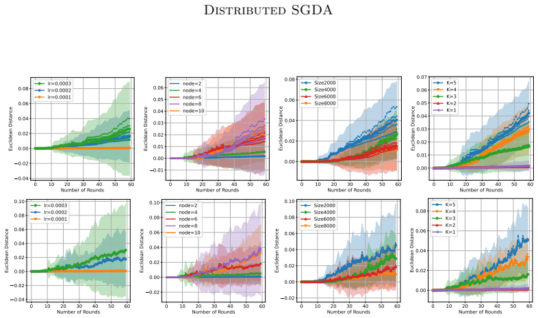
Run Distributed-SGDA on a synthetic PL-strongly-concave minimax problem with parameters chosen so that $\mu^4 \le 32L^2$ or $\rho \le \mu/4$ and measure the excess primal population risk under the paper's decaying schedule; if the stated rate still holds, the hidden condition is unnecessary, and if it does not, the theorem is confined to that regime. Separately, with fixed $\eta$ and varying $K$, measure argument stability on neighbouring datasets to test the predicted $O(\eta K^2)$ growth.
Extended reading notes
Core claim
The central discovery is that the stability of the averaged distributed model can be bounded by a recurring contraction argument whose main input is the consensus term, and that the resulting stability is exactly what controls the generalization gap. Concretely, Theorem 1 proves that $\epsilon$-argument stability implies a weak primal-dual generalization gap at most $\sqrt{2}G\epsilon$, and Theorem 2 proves that under $\mu$-SC-SC local losses with fixed learning rate the argument stability of Distributed-SGDA is at most $\frac{2G(L+\mu)}{L\mu}\left[\eta L\sqrt{\frac{1}{1-\lambda}}\frac{K^2}{2} + \eta L\sqrt{\frac{2\lambda}{(1-\lambda)(1-\lambda^2)}}K^2 + \frac{K}{n}\right]$, so with $\eta \sim 1/(TK)$ the stability is $O((\sqrt{\lambda_1}+\sqrt{\lambda_2})K/T + K/n)$. The same connection yields, under PL-strong-concavity, an excess primal generalization gap and population risk bounded by $O(1/(mn) + (\sqrt{\lambda_1}+\sqrt{\lambda_2})K^{(1+\alpha)/2}/\sqrt{T})$ for $1/2<\alpha<1$, and under nonconvex-nonconcave losses a weak stability bound of $eO((1/n+\sqrt{\lambda_1}+\sqrt{\lambda_2}K^{1/2})^{1/5}(m/n)^{4/5}T^{1/5}K^{3/5})$.
Load-bearing premise
The PL-strongly-concave population-risk bound rests on a hidden condition on the function geometry: the proof requires $\mu^4 > 32L^2$ and $\rho > \mu/4$, and if either fails, the excess primal empirical risk bound that feeds Theorem 7 is not established.
Editorial extensions
If this is right
- With fixed learning rate $\eta$, argument stability of Distributed-SGDA is $O((\sqrt{\lambda_1}+\sqrt{\lambda_2})\eta K^2 + K/n)$, and taking $\eta \sim 1/(TK)$ yields $O((\sqrt{\lambda_1}+\sqrt{\lambda_2})K/T + K/n)$.
- In the PL-strongly-concave case, the excess primal generalization gap and population risk are both $O(1/(mn) + (\sqrt{\lambda_1}+\sqrt{\lambda_2})K^{(1+\alpha)/2}/\sqrt{T})$ for $1/2<\alpha<1$, and the generalization gap dominates the population risk.
- Under nonconvex-nonconcave losses, the weak stability bound of $eO((1/n+\sqrt{\lambda_1}+\sqrt{\lambda_2}K^{1/2})^{1/5}(m/n)^{4/5}T^{1/5}K^{3/5})$ directly implies a weak PD generalization gap via the connection theorem.
- Local-SGDA, obtained by setting $\lambda=0$, recovers the corresponding rates with $\sqrt{\lambda_1}=1$ and $\sqrt{\lambda_2}=0$; Decentralized-SGDA (K=1) matches the earlier rates of Zhu et al. (2023).
Reading between the lines
- Because the proof is modular, the same consensus-plus-expansiveness route should extend to other distributed minimax algorithms such as variance-reduced or momentum variants, provided analogous consensus and contractivity lemmas hold.
- The paper's trade-off analysis implies that hyperparameter search for minimax models should target whichever term dominates the population risk decomposition, a testable prescription for federated GAN training.
- The PL-strongly-concave population-risk result rests on an unstated geometric restriction ($\mu^4 > 32L^2$ and $\rho > \mu/4$); checking whether the stated rates hold outside this regime would delimit or extend Theorem 7.
- Stability bounds of this form typically compose with differential-privacy noise, so a private variant of Local-DSGDA should inherit the same generalization gap plus a privacy term.
Signed reviews
Editorial analysis
A structured set of objections, weighed in public.
Referee Report
Summary. The paper introduces a unified Distributed-SGDA framework that covers Local-SGDA and Local-DSGDA and studies their stability-based generalization. For (strongly) convex--(strongly) concave losses it proves argument-stability bounds and converts them into weak PD generalization and population-risk bounds; for PL--strongly-concave losses it proves primal stability and excess primal population risk; for nonconvex--nonconcave losses it proves weak stability and derives weak PD generalization bounds. The paper also reports preliminary GAN and AUC-maximization experiments. The high-level contribution is a stability-based generalization analysis for local-update and decentralized minimax algorithms, with rates summarized in Tables 1 and 2.
Significance. If the bounds were correct, this would be a useful first systematic stability-based generalization analysis for local-update distributed minimax optimization. The connection theorem between algorithmic stability and the weak PD / excess-primal generalization gaps is a valuable structural contribution, and the paper explicitly identifies the trade-off between generalization gap and optimization error. The analysis is derivation-based rather than parameter-fitting, and the special-case reductions to prior SGDA/DSGDA results are a reasonable consistency check. However, the main stability proofs as written contain a definitional inconsistency and several unstated conditions; until these are repaired, the claimed rates in the tables are not established.
major comments (3)
- [Section 4, Lemma 6, Lemma 7, and Theorem 2] The consensus term is defined as a squared deviation, Δ_t^k = (1/m)Σ_i ||(x_{i,k}−xbar_k, y_{i,k}−ybar_k)||^2, but the proof of Lemma 7 bounds a sum of first powers of such deviations by 2η_t^k L E[Δ_t^k], and the proof of Lemma 6 explicitly writes Δ_t^k as (1/m)Σ_i||...|| without the square before applying Cauchy--Schwarz. Taken literally, Lemma 6 bounds the square root of the quantity that enters the stability recursion, so Theorem 2's recurrence (16) is not derived from the printed definitions. The intended quantity appears to be the average norm, in which case the Cauchy--Schwarz step is acceptable and the final linear-in-η rate is consistent; the definition and all subsequent uses of Δ_t^k must be amended to one convention. Because Theorem 4 and the (S)C-(S)C rows of Tables 1 and 2 all depend on Theorem 2, this inconsistency is load-bearing rather than cosmetic.
- [Theorem 10 and Appendix D.2.1] The potential-function coefficient b = 2μ³L²/(μ⁴−32L²) is used with the requirement b ≤ (ρ−μ/4)μ³/(16L²(L+L²/μ)). This requires μ⁴ > 32L² and ρ > μ/4, but these restrictions are not stated in Theorem 10, in Theorem 7, or in the PL-SC rows of Tables 1 and 2. Since Theorem 7's excess-primal population-risk bound invokes Theorem 10, the PL-SC results are established only under an unstated and quite restrictive parameter regime. The theorem statements should either include these assumptions explicitly and discuss their scope, or the proof should be reworked with a potential function that does not impose them.
- [Theorem 2(ii), Appendix C.1] In the decaying-learning-rate proof, the summation bounds for the three series are justified only under the condition Lμ/(L+μ)(1 + K^{1−α}/(1−α)) > 1. This condition is not stated in Theorem 2(ii) or in Remark 6. Without it, the displayed bound for decaying learning rates does not follow for all admissible K and parameter values. The theorem should state the condition, or the proof should be modified to avoid it.
minor comments (5)
- [Definition 2] The notation E[F(x,y′)] in the weak PD population risk is ambiguous; the expectation should be made explicit over the randomness of the algorithm and the dataset S.
- [Proof of Theorem 1(i), Appendix B] In the chain proving the weak PD generalization gap, one of the two terms is written with Ay(S(r)) on both sides; this appears to be a typo and should read Ay(S) versus Ay(S(r)).
- [Tables 1 and 2] The tilde-O notation eO is used in the table captions and in Remark 6 but is not formally defined; please define it and explicitly state the λ-dependent constants λ1 and λ2 in one place.
- [Algorithm 1] The sample index notation ξ_{i,j_t^k(i)} is used but j_t^k(i) is never defined; please clarify the sampling mechanism for the local stochastic gradients.
- [Experiments, Section 5.2] The experiments are described as preliminary; please state the number of independent runs used to produce the curves, report error bars or confidence intervals, and specify the exact mixing matrices used for the topologies in Figure 2.
Circularity Check
No significant circularity: the stability and generalization bounds are derived from stated assumptions and standard contraction lemmas; the self-citations are technical and not load-bearing.
full rationale
The paper's central claims (Theorems 2, 4, 6-8) are derived through a chain of lemmas from the stated SC-SC/PL-SC/NC-NC assumptions, Lipschitz conditions, and the mixing-matrix spectral parameter. The self-citations to Zhu et al. (2023) are used for standard technical ingredients (Lemma 2, the contraction property of one GDA step; Lemma 3, constants C_lambda) and for comparison benchmarks; these are parameter-free lemmas with explicitly stated assumptions and do not assume the target stability or generalization bounds. The K=1 reduction to the earlier DSGDA rates is consistency, not circularity. No fitted parameter is later relabeled as a prediction, and no uniqueness theorem from the authors is invoked to force a modeling choice. A separate correctness concern exists: Lemma 7 replaces an average of consensus norms by E[Delta_t^k] although Delta is defined as a squared deviation, and Theorem 10's proof imposes an unstated condition on the coefficient b; however, those would be proof gaps or missing assumptions, not circular reasoning. No circular step is established.
Assumptions & free parameters
free parameters (1)
- b =
2µ^3 L^2/(µ^4 - 32L^2)
assumptions (5)
- domain assumption Mixing matrix W is symmetric doubly stochastic with λ < 1.
- domain assumption Each local loss f_i is G-Lipschitz and L-smooth.
- domain assumption Local losses satisfy µ-SC-SC or ρ-PL-µSC conditions.
- ad hoc to paper Parameter b must satisfy b ≤ (ρ - µ/4)µ^3/(16L^2(L + L^2/µ)), which requires µ^4 > 32L^2 and ρ > µ/4.
- ad hoc to paper For decaying learning rates in Theorem 2(ii), Lµ/(L+µ)(1 + K^{1-α}/(1-α)) > 1.
Cite this review
Pith. "Pith review of Stability and Generalization for Distributed SGDA." pith.science (2026). https://pith.science/paper/E7XCPDYK
@misc{pith2026241109365,
  author       = {Pith},
  title        = {Pith review of: Stability and Generalization for Distributed SGDA},
  year         = {2026},
  howpublished = {\url{https://pith.science/paper/E7XCPDYK}},
  note         = {Machine review of arXiv:2411.09365}
}
read the original abstract
Minimax optimization is gaining increasing attention in modern machine learning applications. Driven by large-scale models and massive volumes of data collected from edge devices, as well as the concern to preserve client privacy, communication-efficient distributed minimax optimization algorithms become popular, such as Local Stochastic Gradient Descent Ascent (Local-SGDA), and Local Decentralized SGDA (Local-DSGDA). While most existing research on distributed minimax algorithms focuses on convergence rates, computation complexity, and communication efficiency, the generalization performance remains underdeveloped, whereas generalization ability is a pivotal indicator for evaluating the holistic performance of a model when fed with unknown data. In this paper, we propose the stability-based generalization analytical framework for Distributed-SGDA, which unifies two popular distributed minimax algorithms including Local-SGDA and Local-DSGDA, and conduct a comprehensive analysis of stability error, generalization gap, and population risk across different metrics under various settings, e.g., (S)C-(S)C, PL-SC, and NC-NC cases. Our theoretical results reveal the trade-off between the generalization gap and optimization error and suggest hyperparameters choice to obtain the optimal population risk. Numerical experiments for Local-SGDA and Local-DSGDA validate the theoretical results.
Figures


Reference graph
Works this paper leans on
-
[1]
25 Distributed SGDA For the second term, we proceed as follows: t−1X τ ̸=τ ′ Tr (W τ − Pm)Ξt−τ ktτ T (W τ ′ − Pm)Ξt−τ ′ kt τ ′ ≤ t−1X τ ̸=τ ′ ∥(W τ − Pm)Ξt−τ ktτ ∥F∥(W τ ′ − Pm)Ξt−τ ′ kt τ ′ ∥F ≤ t−1X τ ̸=τ ′ λτ ∥Ξt−τ ktτ ∥F · λτ ′ ∥Ξt−τ ′ kt τ ′ ∥F ≤ 1 2 t−1X τ ̸=τ ′ λτ +τ ′ ∥Ξt−τ ktτ ∥2 F + ∥Ξt−τ ′ kt τ ′ ∥2 F = 1 2 t−1X τ ̸=τ ′ λτ +τ ′ ∥Ξt−τ ktτ ∥2 F +...
work page 2023
-
[4]
Stability and generalization for minibatch sgd and local sgd
Yunwen Lei, Tao Sun, and Mingrui Liu. Stability and generalization for minibatch sgd and local sgd. arXiv preprint arXiv:2310.01139,
-
[7]
For any real-valued matrices A ∈ Rm×n, B ∈ Rn×d, (i) |⟨A, B⟩F| ≤ ∥A∥F∥B∥F; (ii) ∥A∥F ≤ 9A92, and ∥AB∥F ≤ 9A 92 ∥B∥F ≤ ∥A∥F∥B∥F. Lemma 1 (Wang and Joshi 2021). For the mixing matrix W satisfying the Assumption 1, there holds: 9W k − Pm92 = λk, ∀k ∈ N. Lemma 2 (Zhu et al
work page 2021
-
[8]
A.3 Important Lemmas Lemma 3 (Lin et al
For the gradient map Gg,η where g is L-Lipschitz smooth: Gg,η x y = x − η∇xg(x, y) y + η∇yg(x, y) , we have the following expansiveness under different conditions: (i) Gg,η is (1 + ηL)-expansive, i.e., Gg,η x y − Gg,η x′ y′ ≤ (1 + ηL) x − x′ y − y′ ; (ii) When g is µ-strongly-convex-strongly-concave, and the learning rate satisfies η ≤ 2 L+µ , then Gg,η i...
work page 2020
-
[10]
for better understanding and extend existing results to the excess primal generalization gap. Proof of Theorem 1 . Here we set up the distributed neighbouring dataset S, S ′ following these stages. For different datasets S = {S1, ...,Sm} and S ′ = {S ′ 1, ...,S ′ m} with local datasets Si = {ξi,1, ..., ξi,n} and S ′ i = {ξ′ i,1, ..., ξ′ i,n} respectively....
work page 2020
-
[11]
Appendix D. Proof in Nonconvex-Strongly-Concave Case Firstly, we provide some technical lemmas to facilitate our subsequent proof process. D.1 Proof of Stability Proof of Theorem 6 . For distributed neighboring dataset S and S ′, where we assume the each local dataset Si and S ′ i differs at the last sample without loss of generality, i.e., ξi,n 43 Distri...
work page 2022
-
[12]
Proof of Theorem 8 . According to Lemma 7, and substituting condition ( ii) with condi- tion (i) in Lemma 2, we can acquire: EA[ ¯xt k+1 − ¯˙xt k+1 ¯yt k+1 − ¯˙yt k+1 |δt0 k0 = 0] ≤ (1 + ηt kL)EA[ ¯xt k − ¯˙xt k ¯yt k − ¯˙yt k |δt0 k0 = 0] + 2ηt kLEA[∆t k] + 2ηt kG n 51 Distributed SGDA Performing above process from t = T, k= K − 1 to t = t0, k= K − 1, we...
work page 2023
-
[13]
The detailed proof of the equivalence is provided in Example 5.6.6
For simplicity, we omit the subscripts of the ℓ2 norm for vectors and the Frobenius norm for matrices when it does not lead to misunderstanding, i.e., ∥x∥ denotes ∥x∥2 and ∥A∥ means ∥A∥F. The detailed proof of the equivalence is provided in Example 5.6.6. in (Horn and Johnson, 2012). Property 2 (Horn and Johnson
work page 2012
Show all 12 references
-
[2002]
Proximal gradient descent-ascent: Variable convergence under k {\L} geometry
Ziyi Chen, Yi Zhou, Tengyu Xu, and Yingbin Liang. Proximal gradient descent-ascent: Variable convergence under k {\L} geometry. arXiv preprint arXiv:2102.04653,
-
[2012]
Efficient algorithms for federated saddle point optimization
Charlie Hou, Kiran K Thekumparampil, Giulia Fanti, and Sewoong Oh. Efficient algorithms for federated saddle point optimization. arXiv preprint arXiv:2102.06333,
-
[2021]
Linear convergence of gradient and proximal-gradient methods under the polyak-lojasiewicz condition
Hamed Karimi, Julie Nutini, and Mark Schmidt. Linear convergence of gradient and proximal-gradient methods under the polyak-lojasiewicz condition. In Machine Learning and Knowledge Discovery in Databases: European Conference, ECML PKDD 2016, Riva del Garda, Italy, September 19...
2016
-
[2023]
Stochastic smoothed gradient descent ascent for federated minimax optimization
Wei Shen, Minhui Huang, Jiawei Zhang, and Cong Shen. Stochastic smoothed gradient descent ascent for federated minimax optimization. arXiv preprint arXiv:2311.00944,
Reviewed August 12, 2026 · model on record in the stance chip above.
Discussion (0). Continue with ORCID to comment.