Multimodal sampling via Schr\"odinger-F\"ollmer samplers with temperatures

Xiaojie Wang; Xiaoyan Zhang

REVIEW 2 major objections 3 minor 44 references

Multimodal sampling via Schr\"odinger-F\"ollmer samplers with temperatures

T0 review · 2 major / 3 minor · reviewed 2026-08-03 · deepseek-v4-flash

Challenge this review Re-run · record.json Download PDF Read on arXiv ↗

Pith's one-line read Introducing a temperature parameter into Schrödinger–Föllmer samplers cuts their Euler-discretization error from O(√h) to O(h) in Wasserstein distance, without convexity or ergodicity requirements.

desk verdict Genuine O(h) upgrade for exact-drift Schrödinger–Föllmer samplers, but the Monte-Carlo half of the paper has a real, fixable flaw in Theorem 3.7. read the letter →

arxiv 2512.23965 v2 pith:FHGHSNGN submitted 2025-12-30 math.NA cs.NA

Xiaojie Wang , Xiaoyan Zhang This is my paper

classification math.NAcs.NA MSC 60H3565C0565C30

keywords Schrödinger-FöllmersamplertemperatureparameterEuler-MaruyamadiscretizationL2-WassersteindistancemultimodalsamplingMonteCarlodriftapproximationnon-convexgradient-free

verification ladder T0 review T1 audit T2 compute T3 formal

The pith

A machine-rendered reading of the paper's core claim, the machinery that carries it, and where it could break.

The reading

Sampling from a high-dimensional, multimodal target usually requires an ergodic diffusion that runs long enough to mix, and mixing can fail when modes are separated by energy barriers. This paper instead transports a point mass to the target over the unit interval via a Schrödinger–Föllmer diffusion with a temperature parameter β, and analyzes a plain Euler discretization of that bridge. Its central claim is that the discretized sampler converges in L2-Wasserstein distance at rate O(h) for the exact drift, and at O(h)+O(√(d/M)) when the drift is Monte-Carlo-estimated — a full order better than the earlier O(√h) bound, with no convexity or ergodicity assumed. A sympathetic reader would take the main payoff to be practical: a gradient-free sampler that provably needs fewer drift evaluations for a given Wasserstein tolerance, plus a temperature knob that numerically lets the sampler cross between modes instead of collapsing onto one.

What carries the argument

The load-bearing object is the temperature-parameterized Schrödinger–Föllmer diffusion (2.7), whose drift f_β(x,t) = β ∇ log(Q^β_{1−t}g_β(x)) is built from the density ratio g_β = dμ/dN(0,βI_d) and its heat-semigroup smoothing. This process connects δ_0 at t=0 to μ at t=1 without ergodicity, and β rescales drift and noise together, which is what lets the sampler explore across modes. The proof machinery is a refined Euler-error decomposition: the authors use Itô's formula to expand f_β(X_s,s) − f_β(X_{t_{i−1}},t_{i−1}) and bound the four resulting terms using the integrable singularity ‖∂_t f_β(x,t)‖ ≤ L̃_f d^{1/2}/√(1−t); that bound is the reason the Wasserstein error becomes O(h) rather th

What would settle it

Take a target whose density ratio g_β has genuinely heavy tails (so the lower bound g_β ≥ ρ fails), for example a single Gaussian with small variance at β=1, run the Euler scheme (3.1) with exact drift for step sizes h=2^{−5},…,2^{−9}, and measure W2(Law(Y_1), μ) by Monte Carlo; if the error decays like h^{1/2} rather than h, the theorem's assumptions are not merely technical. A cleaner check is to verify the integrable-singularity bound (3.3) directly for that target's drift.

Watch

Extended reading notes

Core claim

The paper's central discovery is that the temperature-scaled Schrödinger–Föllmer process dX_t = f_β(X_t,t) dt + √β dW_t, with drift f_β = β ∇ log(Q^β_{1−t} g_β), still transports δ_0 to the target μ at time 1, and does so in a way amenable to first-order discretization analysis. Under smoothness of the drift and a positive lower bound on the density ratio g_β, the authors prove for the Euler–Maruyama scheme with exact drift that W2(Law(Y_1), μ) ≤ C d h, and for the scheme with an M-sample Monte Carlo drift that W2(Law(Ỹ^M_1), μ) ≤ C d h + C √(d/M). The temperature parameter does more than generalize the earlier β=1 case: numerical experiments show that higher β is what allows the sampler to

Load-bearing premise

The O(h) rate rests on Assumption 3.1 — the drift's time derivative obeys ‖∂_t f_β(x,t)‖ ≤ L̃_f d^{1/2}/√(1−t) — together with the positive lower bound g_β ≥ ρ > 0; if either fails for a target, the enhanced first-order error bound is not proven and the earlier √h-type behavior may reappear.

Editorial extensions

If this is right

With exact drift, the order-one bound W2 ≤ C d h means a target Wasserstein accuracy ϵ needs only O(d/ϵ) drift evaluations and Brownian increments, a quadratic-to-linear improvement over the earlier O(d/ϵ²) cost.
With the Monte Carlo drift, the bound W2 ≤ C d h + C√(d/M) means the same Gaussian samples can be generated once and reused at every time step, reducing MC cost to O(M) rather than O(N·M).
The convergence analysis requires neither convexity nor a log-Sobolev inequality nor ergodicity, so the sampler is applicable to non-log-concave targets where Langevin-style guarantees typically need extra mixing assumptions.
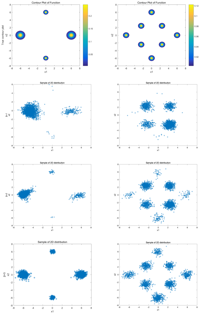
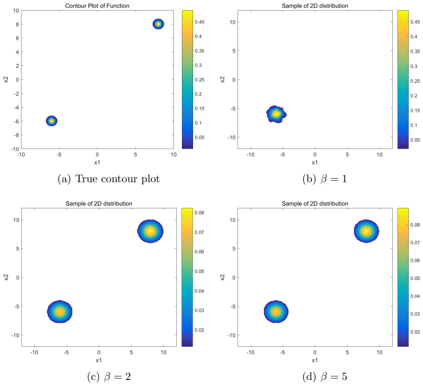
Numerical experiments show the temperature parameter β directly controls mode exploration: β=1 can miss modes of Gaussian mixtures, while β=2 or 5 recovers all modes without changing the target at time 1.
The empirical mean-square convergence rates for Gaussian mixtures and Bayesian ridge regression are close to order one, consistent with the theorems.

Reading between the lines

Editorial extensions of the paper, not claims the author makes directly.

An implication the paper leaves implicit is an annealing reading: increasing β flattens the effective potential in g_β ∝ exp(−V(x)+‖x‖²/(2β)), so the 'temperature' is doing the same barrier-crossing work as in simulated tempering; this suggests a time-varying β(t) schedule could combine exploration at high β with accuracy at low β, a mechanism not analyzed here.
The theory assumes g_β ≥ ρ > 0, but two of the paper's own shaped-distribution experiments (p₁ and p₃ at β=1) have density ratios that are unbounded above and decay to zero in the tails, so those experiments demonstrate robustness beyond the theorem's assumptions rather than a verified regime.
Because the sampler is gradient-free and runs on a fixed interval [0,1], it resembles a diffusion-model-style transport map; a natural testable variant would replace the Monte Carlo drift with a learned or adaptive estimator and check whether the O(h) discretization rate survives, but that is outside this paper.
The dimension dependence d in the O(dh) bound is worse than the √d or dimension-free rates common for log-concave Langevin analysis; a refined analysis might trade the strong smoothness assumption for a smaller dimension factor, but the paper does not attempt this.

Share X Bluesky LinkedIn Reddit HN

Editorial analysis

A structured set of objections, weighed in public.

Desk editor's note, referee report, and a circularity audit.

Desk Editor's Note

read the letter

Colleague,

Quick take: this is a genuine upgrade to the SFS line in [21], but only the exact-drift half is fully solid. The temperature-parameterized process and the O(h) Wasserstein analysis for the exact-drift Euler scheme are new, and the proof carries weight: the Itô expansion handling the integrably singular ∂_t f_β is legitimate and the T1–T4 split is coherent. If you work on Schrödinger–Föllmer samplers, read Section 4.1. Theorem 3.4's bound W2 ≤ C d h is the paper's real contribution.

What else it does well: the reuse-once Monte Carlo input saving for the inexact sampler is a real practical improvement, and the numerical section honestly shows that high temperature avoids mode collapse. That effect is empirical, but presented as such.

Where it gets soft: Theorem 3.7. Equation (3.10) defines the Monte Carlo drift by two expressions that are equal only in expectation. The first is a ratio of sample means of ∇g and g; the second replaces ∇g via Stein using a sample mean of ξ g multiplied by 1/sqrt((1−t)β). For finite M they are not the same estimator. The proof uses the second, gradient-free form and Lemma 4.2, which asserts a t-uniform O(d/M) bound. But that form has a singular denominator near t=1. A delta-method computation at t=1−h gives variance of order d/(hM), not d/M. So Lemma 4.2 cannot hold t-uniformly for the estimator as written, the J2 term in (4.15) picks up at least log(1/h), and Theorem 3.7 as stated does not follow from the given proof. Citing [21, Lemma A.6] does not repair it: that lemma bounds the ∇g-form, which has no such denominator. This is a load-bearing flaw in one of the two headline theorems. It looks fixable—use the ∇g-form, or prove a t-dependent MC bound—but it is not cosmetic.

Smaller issues: the convergence-rate experiments in Section 5 measure self-consistency against a fine-step numerical solution rather than W2 to the target; the p1/p3 examples in Section 5.1 run at β=1 where g_β is unbounded and violates the lower-bound assumption (2.11), so those figures are extrapolations; and the mode-recovery plots have no error bars. None of these touches Theorem 3.4.

Verdict: the paper deserves a serious referee. The exact-drift O(h) result alone justifies it, and the MC flaw is addressable. I would send it out and ask the referee to focus on the estimator discrepancy and on t-uniformity of Lemma 4.2.

Referee Report

2 major / 3 minor

Summary. The paper introduces a temperature parameter β into the Schrödinger–Föllmer diffusion, studies Euler samplers with exact and Monte Carlo drift, and claims W2 error bounds of order O(dh) for the exact-drift sampler (Theorem 3.4) and O(dh + sqrt(d/M)) for the Monte-Carlo-drift sampler (Theorem 3.7), without convexity or ergodicity assumptions. Numerical experiments illustrate the benefit of high temperatures for multimodal targets. The proof of Theorem 3.4 is a genuinely new analysis: it expands the drift increment by Itô's formula and uses the integrable singularity of ∂_t fβ to upgrade the previous O(sqrt(h)) rate. However, the proof of Theorem 3.7 rests on a Monte-Carlo error bound that is not valid for the gradient-free estimator displayed in Eq. (3.10), so the second main theorem is currently unsupported as stated.

Significance. If Theorem 3.4 stands, it is a substantial improvement over the O(sqrt(h)) rate of Huang et al. [21] for Schrödinger–Föllmer samplers, and the technique of handling the terminal singularity of ∂_t fβ by Itô expansion is a useful contribution. The temperature mechanism is also empirically attractive for multimodal sampling. The exact-drift result appears internally coherent and the T1–T4 estimates in Section 4.1 are plausible. The Monte-Carlo-drift theorem, however, is not: the estimator in Eq. (3.10) is ambiguous, and for the natural gradient-free form the uniform O(d/M) variance bound of Lemma 4.2 is false, with variance growing like 1/(1−t). This affects a central advertised result and requires major revision.

major comments (2)

[§3.2] The two expressions in (3.10) are not equal for finite M. Stein's lemma gives an identity between expectations, not between sample averages. For the second, gradient-free estimator, at t_n=1−h one has \hat f^M ≈ β/(√(hβ)) · (1/M)Σ_j ξ_j g(x+√(hβ)ξ_j)/( (1/M)Σ_j g(...) ) ≈ √(β/h) · (1/M)Σ_j ξ_j as h→0, giving E||\hat f^M − f||² = O(β d/(hM)). Thus Lemma 4.2's uniform-in-n bound O(d/M) is false for this estimator, and the J2 estimate in (4.15) misses at least a log(1/h) factor after summation. The citation to [21, Lemma A.6] is insufficient, especially because that lemma, if it concerns the ∇g-form, lacks the singular 1/√(1−t) denominator. The authors must specify exactly which estimator is used, provide a self-contained proof of the relevant t-uniform MC bound, or revise the MC term in Theorem 3.7. Proposition 3.6's uniform Lipschitz bound is also only plausible for the first, ∇g-based ex
[§5.1/§5.2] The numerical experiments systematically run the sampler outside the assumptions of the theorems. For p1 and p3 at β=1, g1 is proportional to exp((8x1+8x2−x1²x2²)/2) and exp(2αx1), both unbounded; for p2, g1 decays to 0 as r→∞. Hence Assumption 2.2 (gβ ≥ ρ > 0) fails for all three shaped distributions. The Gaussian-mixture examples with covariance Σi=1/5 I_d, 1/4 I_d, or 4/5 I_d at β=1 also have gβ → 0 at infinity, so the lower-bound assumption fails there as well. The paper suggests a regularization in Section 3.1 but does not use it in the numerics. This should be explicitly acknowledged as extrapolation; otherwise the numerical sections do not confirm the theorems under the stated hypotheses.

minor comments (3)

[§4.1, after Eq. (4.12)] The sentence 'The proof of Theorem 3.7 is completed' should refer to Theorem 3.4.
[Throughout] Typos: 'dose not' in §3.1 and §3.2; 'geven' in Lemma 2.4; 'Schr¨ odinger' spacing in the references. A light proofreading pass is needed.
[§3.2] The statement 'M independent Gaussian random variables are only generated once and repeatedly used' is a useful algorithmic detail, but the paper should clarify how this interacts with the MC variance bound in Lemma 4.2, since the ξ_j are not refreshed at each time step.

Circularity Check

0 steps flagged · score 0.0 of 10

No significant circularity: the O(h) bounds are derived from explicit assumptions and external lemmas; self-citations are not load-bearing.

full rationale

The paper's central derivation is self-contained rather than circular. Theorem 3.4 bounds the Euler discretization error by first writing the remainder R_i in (4.2), applying Itô's formula, and then using Assumption 3.1 — in particular the integrable singularity bound (3.3) — together with Hölder, Itô isometry, and discrete Gronwall. The O(h) rate is obtained, not assumed as the conclusion. Proposition 3.2 verifies Assumption 3.1 from primitive smoothness and lower-bound conditions on g_beta, and Proposition 3.3 gives sufficient conditions on V; these are forward assumptions, not definitions of the target result. Theorem 3.7 adds the Monte-Carlo drift error through Lemma 4.2, which is referred to the external result [21, Lemma A.6]; even if the uniformity of that lemma were questionable, that would be a proof gap rather than a self-referential reduction. No fitted parameters are renamed as predictions, no uniqueness theorem is imported from the authors' own prior work, and no ansatz is smuggled in through self-citation. The citations [30] and [42] appear only as statements about ongoing projects and carry no weight in the proofs. The temperature experiments are empirical demonstrations, not presented as consequences forced by assumptions. Therefore no circular step is exhibited.

Assumptions & free parameters 1 free parameters · 5 assumptions · 1 invented entities

The central claims rest on: (a) the ρ-lower-bound and Lipschitz conditions on the density ratio g_β; (b) the singular time-derivative bound (3.3), which is the mechanism for O(h); (c) imported lemmas from [21] (well-posedness, moment bounds, uniform MC variance). No constants are fitted to data; β is a user-selected hyperparameter. The main ledger risk is the t-uniform MC-variance lemma applied to an estimator whose Stein form is singular near t=1.

free parameters (1)

Temperature β = β = 1, 2, 5 in numerical experiments; arbitrary β > 0 in theory
User-chosen hyperparameter. The qualitative finding that large β avoids mode collapse is selected by experiment, not predicted by the theory, which is stated uniformly in β with β-independent constants.

assumptions (5)

domain assumption g_β ≥ ρ > 0 and g_β, ∇g_β are L_g-Lipschitz (Assumption 2.2)
Needed for well-posedness (Prop. 2.3), drift Lipschitzness, and the Monte-Carlo error bound (Lemma 4.2). Restrictive; the paper offers an ρ-mixing remedy (§3.1) that its own numerical examples do not use.
domain assumption Drift smoothness and singular time-derivative bound ‖∂_t f_β(x,t)‖ ≤ L̃_f d^{1/2}/√(1−t) (Assumption 3.1, eq. (3.3))
The load-bearing condition that upgrades the rate from √h to h; verified (Prop. 3.2) only under C³ + Lipschitz + lower-bound conditions that the p₁/p₃ examples in §5.1 violate for β=1.
domain assumption Well-posedness and X₁ ∼ μ of (2.7) (Prop. 2.3, via [21, Appendix B])
Borrowed from [21] without proof; asserts the diffusion transports δ₀ at t=0 to the target μ at t=1.
domain assumption Uniform Monte-Carlo variance bound E^ξ‖f_β − f̃^M_β‖² ≤ C₂d/M (Lemma 4.2, cited to [21, Lemma A.6])
Applied at every grid point including t→1, but the estimator (3.10) in Stein-lemma form divides by √((1−t)β); its variance appears to scale like βd/(M(1−t)) near t=1. The t-uniform bound is asserted, not derived in this text.
standard math Stein’s lemma, Itô formula, Itô isometry, discrete Gronwall, moment bounds (Lemma 2.4 via [21, Lemmas A.3–A.4])
Standard tools; Lemma 2.4 and the well-posedness result are cited from [21] rather than proved here.

invented entities (1)

Temperature-parameterized Schrödinger–Föllmer process (2.7) and samplers (3.1)/(3.11)
purpose: Finite-time bridge from δ₀ to μ with tunable noise/drift scaling, intended to ease crossing between modes of multimodal targets.
A new mathematical object within the paper; its usefulness rests on the paper’s own theorems and numerical demonstrations, with no external falsifiable prediction attached.

how reviews work

0 comments

Cite this review

Pith. "Pith review of Multimodal sampling via Schr\"odinger-F\"ollmer samplers with temperatures." pith.science (2026). https://pith.science/paper/FHGHSNGN

@misc{pith2026251223965,
  author       = {Pith},
  title        = {Pith review of: Multimodal sampling via Schr\"odinger-F\"ollmer samplers with temperatures},
  year         = {2026},
  howpublished = {\url{https://pith.science/paper/FHGHSNGN}},
  note         = {Machine review of arXiv:2512.23965}
}

abstract

Generating samples from complex and high-dimensional distributions is ubiquitous in various scientific fields of statistical physics, Bayesian inference, scientific computing and machine learning. Very recently, Huang et al. (IEEE Trans. Inform. Theory, 2025) proposed new Schr\"odinger-F\"ollmer samplers (SFS), based on the Euler discretization of the Schr\"odinger-F\"ollmer diffusion evolving on the unit interval $[0, 1]$. There, a convergence rate of order $\mathcal{O}(\sqrt{h})$ in the $L^2$-Wasserstein distance was obtained for the Euler discretization with a uniform time step-size $h>0$. By introducing a temperature parameter, different samplers are proposed in this paper, based on the Euler discretization of the Schr\"odinger-F\"ollmer process with temperatures. As revealed by numerical experiments, high temperatures are vital, particularly in sampling from multimodal distributions. Further, a novel approach of error analysis is developed for the time discretization and an enhanced convergence rate of order $\mathcal{O}(h)$ is obtained in the $L^2$-Wasserstein distance, under certain smoothness conditions on the drift. This significantly improves the existing order-half convergence in the aforementioned paper. Unlike Langevin samplers, SFS is gradient-free, works in a unit interval $[0, 1]$ and does not require any ergodicity. Numerical experiments confirm the convergence rate and show that, the SFS substantially outperforms vanilla Langevin samplers, particularly in sampling from multimodal distributions.

Figures

Figures reproduced from arXiv: 2512.23965 by the authors.

**Figure 2.** Sampling from p2(x) with SFS [PITH_FULL_IMAGE:figures/full_fig_p020_2.png] view at source ↗

**Figure 3.** Sampling from p3(x) with SFS. 20 [PITH_FULL_IMAGE:figures/full_fig_p020_3.png] view at source ↗

Figures from the paper (7 more)

**Figure 4.** Figure 4: Probability density of the one-dimensional Gaussian mixture distribution. [PITH_FULL_IMAGE:figures/full_fig_p021_4.png]

**Figure 5.** Figure 5: Sampling via SFS, Overdamped LMC, and BAOAB. [PITH_FULL_IMAGE:figures/full_fig_p023_5.png]

**Figure 6.** Figure 6: Sampling via SFS with different temperatures [PITH_FULL_IMAGE:figures/full_fig_p024_6.png]

**Figure 7.** Figure 7: Sampling via SFS with different temperatures [PITH_FULL_IMAGE:figures/full_fig_p025_7.png]

**Figure 8.** Figure 8: Probability density of the first component of the Gaussian mixture distribution. [PITH_FULL_IMAGE:figures/full_fig_p026_8.png]

**Figure 9.** Figure 9: Mean-square convergence rates of SFS algorithms for the Gaussian mixture distributions. [PITH_FULL_IMAGE:figures/full_fig_p027_9.png]

**Figure 10.** Figure 10: Mean-square convergence rates of SFS algorithm for the Bayesian ridge regression. [PITH_FULL_IMAGE:figures/full_fig_p027_10.png]

Discussion (0). Sign in to comment.

Reference graph

Works this paper leans on

44 extracted references · 7 linked inside Pith

[21]

Schr¨ odinger-F¨ ollmer sampler.IEEE Trans

Jian Huang, Yuling Jiao, Lican Kang, Xu Liao, Jin Liu, and Yanyan Liu. Schr¨ odinger-F¨ ollmer sampler.IEEE Trans. Inform. Theory, 71(2):1283–1299, 2025

2025
[1]

Stochastic interpolants: A unifying framework for flows and diffusions.arXiv preprint arXiv:2303.08797, 2023

Michael S Albergo, Nicholas M Boffi, and Eric Vanden-Eijnden. Stochastic interpolants: A unifying framework for flows and diffusions.arXiv preprint arXiv:2303.08797, 2023

arXiv 2023
[2]

Building Normalizing Flows with Stochas- tic Interpolants.In International Conference on Learning Representations, 2023

Michael Samuel Albergo and Eric Vanden-Eijnden. Building Normalizing Flows with Stochas- tic Interpolants.In International Conference on Learning Representations, 2023

2023
[3]

Altschuler and Sinho Chewi

Jason M. Altschuler and Sinho Chewi. Shifted Composition III: Local Error Framework for KL Divergence.ArXiv, abs/2412.17997, 2024

arXiv 2024
[4]

Second order quantitative bounds for unadjusted generalized Hamiltonian Monte Carlo.arXiv preprint arXiv:2306.09513, 2023

Evan Camrud, Alain Durmus, Pierre Monmarch´ e, and Gabriel Stoltz. Second order quantitative bounds for unadjusted generalized Hamiltonian Monte Carlo.arXiv preprint arXiv:2306.09513, 2023

arXiv 2023
[5]

Improved analysis of score-based generative modeling: User-friendly bounds under minimal smoothness assumptions

Hongrui Chen, Holden Lee, and Jianfeng Lu. Improved analysis of score-based generative modeling: User-friendly bounds under minimal smoothness assumptions. InInternational Conference on Machine Learning, pages 4735–4763. PMLR, 2023

2023
[6]

Zongchen Chen and Santosh S. Vempala. Optimal convergence rate of Hamiltonian Monte Carlo for strongly logconcave distributions.Theory Comput., 18:Paper No. 9, 18, 2022

2022
[7]

Sharp convergence rates for Langevin dynamics in the nonconvex setting.arXiv preprint arXiv:1805.01648, 2018

Xiang Cheng, Niladri S Chatterji, Yasin Abbasi-Yadkori, Peter L Bartlett, and Michael I Jordan. Sharp convergence rates for Langevin dynamics in the nonconvex setting.arXiv preprint arXiv:1805.01648, 2018

arXiv 2018

Show all 44 references

[8]

Underdamped Langevin MCMC: A non-asymptotic analysis

Xiang Cheng, Niladri S Chatterji, Peter L Bartlett, and Michael I Jordan. Underdamped Langevin MCMC: A non-asymptotic analysis. InConference on learning theory, pages 300–
[9]

Global optimization via Schr¨ odinger-F¨ ollmer diffusion.SIAM J

Yin Dai, Yuling Jiao, Lican Kang, Xiliang Lu, and Jerry Zhijian Yang. Global optimization via Schr¨ odinger-F¨ ollmer diffusion.SIAM J. Control Optim., 61(5):2953–2980, 2023

2023
[10]

Dalalyan

Arnak S. Dalalyan. Theoretical guarantees for approximate sampling from smooth and log- concave densities.J. R. Stat. Soc. Ser. B. Stat. Methodol., 79(3):651–676, 2017

2017
[11]

Dalalyan and Avetik Karagulyan

Arnak S. Dalalyan and Avetik Karagulyan. User-friendly guarantees for the Langevin Monte Carlo with inaccurate gradient.Stochastic Process. Appl., 129(12):5278–5311, 2019. 28

2019
[12]

Dalalyan and Lionel Riou-Durand

Arnak S. Dalalyan and Lionel Riou-Durand. On sampling from a log-concave density using kinetic Langevin diffusions.Bernoulli, 26(3):1956–1988, 2020

1956
[13]

Nonasymptotic convergence analysis for the unadjusted Langevin algorithm.Ann

Alain Durmus and ´Eric Moulines. Nonasymptotic convergence analysis for the unadjusted Langevin algorithm.Ann. Appl. Probab., 27(3):1551–1587, 2017

2017
[14]

High-dimensional Bayesian inference via the unadjusted Langevin algorithm.Bernoulli, 25(4A):2854–2882, 2019

Alain Durmus and ´Eric Moulines. High-dimensional Bayesian inference via the unadjusted Langevin algorithm.Bernoulli, 25(4A):2854–2882, 2019

2019
[15]

Reflection couplings and contraction rates for diffusions.Probab

Andreas Eberle. Reflection couplings and contraction rates for diffusions.Probab. Theory Related Fields, 166(3-4):851–886, 2016

2016
[16]

Random fields and diffusion processes.Lect

Hans F¨ ollmer. Random fields and diffusion processes.Lect. Notes Math, 1362:101–204, 1988

1988
[17]

An entropy approach to the time reversal of diffusion processes

Hans F¨ ollmer. An entropy approach to the time reversal of diffusion processes. InStochas- tic Differential Systems Filtering and Control: Proceedings of the IFIP-WG 7/1 Working Conference Marseille-Luminy, France, March 12–17, 1984, pages 156–163. Springer, 2005

1984
[18]

OUP Oxford, 2002

Paul H Garthwaite, Ian T Jolliffe, and Byron Jones.Statistical inference. OUP Oxford, 2002

2002
[19]

Michael B. Giles. Multilevel Monte Carlo path simulation.Oper. Res., 56(3):607–617, 2008

2008
[20]

Multilevel monte carlo methods

Stefan Heinrich. Multilevel monte carlo methods. InInternational Conference on Large-Scale Scientific Computing, pages 58–67. Springer, 2001

2001
[22]

World Scientific Publishing Company, 2012

Fima C Klebaner.Introduction to stochastic calculus with applications. World Scientific Publishing Company, 2012

2012
[23]

A randomized Milstein method for stochastic differential equa- tions with non-differentiable drift coefficients.Discrete Contin

Raphael Kruse and Yue Wu. A randomized Milstein method for stochastic differential equa- tions with non-differentiable drift coefficients.Discrete Contin. Dyn. Syst. Ser. B, 24(8):3475– 3502, 2019

2019
[24]

Approximation of expectation of diffusion process and mathematical finance

Shigeo Kusuoka. Approximation of expectation of diffusion process and mathematical finance. InTaniguchi Conference on Mathematics Nara ’98, volume 31 ofAdv. Stud. Pure Math., pages 147–165. Math. Soc. Japan, Tokyo, 2001

2001
[25]

Representation formula for the entropy and functional inequalities.Ann

Joseph Lehec. Representation formula for the entropy and functional inequalities.Ann. Inst. Henri Poincar´ e Probab. Stat., 49(3):885–899, 2013

2013
[26]

Rational construction of stochastic numerical methods for molecular sampling.Appl

Benedict Leimkuhler and Charles Matthews. Rational construction of stochastic numerical methods for molecular sampling.Appl. Math. Res. Express. AMRX, (1):34–56, 2013

2013
[27]

Mattingly, and Lihan Wang

Lei Li, Jianfeng Lu, Jonathan C. Mattingly, and Lihan Wang. Numerical methods for stochas- tic differential equations based on Gaussian mixture.Commun. Math. Sci., 19(6):1549–1577, 2021. 29

2021
[28]

A sharp uniform-in-time error estimate for Stochastic Gradient Langevin Dynamics.arXiv preprint arXiv:2207.09304, 2022

Lei Li and Yuliang Wang. A sharp uniform-in-time error estimate for Stochastic Gradient Langevin Dynamics.arXiv preprint arXiv:2207.09304, 2022

2022 arXiv
[29]

Sqrt (d) dimension Dependence of Langevin Monte Carlo

Ruilin Li, Hongyuan Zha, and Molei Tao. Sqrt (d) dimension Dependence of Langevin Monte Carlo. InThe International Conference on Learning Representations, 2022

2022
[30]

Accelerating the Schr¨ odinger-F¨ ollmer diffu- sion based multimodal sampling via stochastic Runge-Kutta.Preprint, 2025

Haotian Lin, Xiaojie Wang, and Xiaoyan Zhang. Accelerating the Schr¨ odinger-F¨ ollmer diffu- sion based multimodal sampling via stochastic Runge-Kutta.Preprint, 2025

2025
[31]

Cubature on wiener space.Proceedings of the Royal Society of London

Terry Lyons and Nicolas Victoir. Cubature on wiener space.Proceedings of the Royal Society of London. Series A: Mathematical, Physical and Engineering Sciences, 460(2041):169–198, 2004
[32]

Elsevier, 2007

Xuerong Mao.Stochastic differential equations and applications. Elsevier, 2007

2007
[33]

High-dimensional MCMC with a standard splitting scheme for the un- derdamped Langevin diffusion.Electron

Pierre Monmarch´ e. High-dimensional MCMC with a standard splitting scheme for the un- derdamped Langevin diffusion.Electron. J. Stat., 15(2):4117–4166, 2021

2021
[34]

Wainwright, and Peter L

Wenlong Mou, Nicolas Flammarion, Martin J. Wainwright, and Peter L. Bartlett. Im- proved bounds for discretization of Langevin diffusions: near-optimal rates without convexity. Bernoulli, 28(3):1577–1601, 2022

2022
[35]

Springer Science & Business Media, 2013

Bernt Oksendal.Stochastic differential equations: an introduction with applications. Springer Science & Business Media, 2013

2013
[36]

Projected Langevin Monte Carlo algorithms in non-convex and super-linear setting.J

Chenxu Pang, Xiaojie Wang, and Yue Wu. Projected Langevin Monte Carlo algorithms in non-convex and super-linear setting.J. Comput. Phys., 526:Paper No. 113754, 33, 2025

2025
[37]

John Wiley & Sons, 2016

Reuven Y Rubinstein and Dirk P Kroese.Simulation and the Monte Carlo method. John Wiley & Sons, 2016

2016
[38]

Unbiased estimation using a class of diffusion processes.J

Hamza Ruzayqat, Alexandros Beskos, Dan Crisan, Ajay Jasra, and Nikolas Kantas. Unbiased estimation using a class of diffusion processes.J. Comput. Phys., 472:Paper No. 111643, 21, 2023

2023
[39]

Sur la th´ eorie relativiste de l’´ electron et l’interpr´ etation de la m´ ecanique quantique

Erwin Schr¨ odinger. Sur la th´ eorie relativiste de l’´ electron et l’interpr´ etation de la m´ ecanique quantique. InAnnales de l’institut Henri Poincar´ e, volume 2, pages 269–310, 1932

1932
[40]

Convergence of kinetic Langevin samplers for non- convex potentials.arXiv preprint arXiv:2405.09992, 2024

Katharina Schuh and Peter A Whalley. Convergence of kinetic Langevin samplers for non- convex potentials.arXiv preprint arXiv:2405.09992, 2024

2024 arXiv
[41]

Theoretical guarantees for sampling and inference in generative models with latent diffusions

Belinda Tzen and Maxim Raginsky. Theoretical guarantees for sampling and inference in generative models with latent diffusions. InConference on Learning Theory, pages 3084–
[42]

When Schr¨ odinger-F¨ ollmer samplers meet randomization: order one convergence with sqrt(d) dimension dependence.Preprint, 2025

Xiaojie Wang and Xiaoyan Zhang. When Schr¨ odinger-F¨ ollmer samplers meet randomization: order one convergence with sqrt(d) dimension dependence.Preprint, 2025. 30

2025
[43]

Bin Yang and Xiaojie Wang. Non-asymptotic Error Bounds inW 2-Distance with Sqrt(d) Dimension Dependence and First Order Convergence for Langevin Monte Carlo beyond Log- Concavity.International Conference on Machine Learning, 2025

2025
[44]

Stochastic Transport Maps in Diffusion Models and Sampling.arXiv preprint arXiv:2503.20573, 2025

Xicheng Zhang. Stochastic Transport Maps in Diffusion Models and Sampling.arXiv preprint arXiv:2503.20573, 2025. A Proof of Proposition 3.2 Proof.Under the given assumptions, the functiong β is of classC 3, and moreover,g β,∇g β,∇ 2gβ are Lipschitz continuous. Then there exist...

2025 arXiv

Pith tools

Reviewed August 3, 2026 · model on record in the stance chip above.

[1] [21]

Schr¨ odinger-F¨ ollmer sampler.IEEE Trans

Jian Huang, Yuling Jiao, Lican Kang, Xu Liao, Jin Liu, and Yanyan Liu. Schr¨ odinger-F¨ ollmer sampler.IEEE Trans. Inform. Theory, 71(2):1283–1299, 2025

2025

[2] [1]

Stochastic interpolants: A unifying framework for flows and diffusions.arXiv preprint arXiv:2303.08797, 2023

Michael S Albergo, Nicholas M Boffi, and Eric Vanden-Eijnden. Stochastic interpolants: A unifying framework for flows and diffusions.arXiv preprint arXiv:2303.08797, 2023

arXiv 2023

[3] [2]

Building Normalizing Flows with Stochas- tic Interpolants.In International Conference on Learning Representations, 2023

Michael Samuel Albergo and Eric Vanden-Eijnden. Building Normalizing Flows with Stochas- tic Interpolants.In International Conference on Learning Representations, 2023

2023

[4] [3]

Altschuler and Sinho Chewi

Jason M. Altschuler and Sinho Chewi. Shifted Composition III: Local Error Framework for KL Divergence.ArXiv, abs/2412.17997, 2024

arXiv 2024

[5] [4]

Second order quantitative bounds for unadjusted generalized Hamiltonian Monte Carlo.arXiv preprint arXiv:2306.09513, 2023

Evan Camrud, Alain Durmus, Pierre Monmarch´ e, and Gabriel Stoltz. Second order quantitative bounds for unadjusted generalized Hamiltonian Monte Carlo.arXiv preprint arXiv:2306.09513, 2023

arXiv 2023

[6] [5]

Improved analysis of score-based generative modeling: User-friendly bounds under minimal smoothness assumptions

Hongrui Chen, Holden Lee, and Jianfeng Lu. Improved analysis of score-based generative modeling: User-friendly bounds under minimal smoothness assumptions. InInternational Conference on Machine Learning, pages 4735–4763. PMLR, 2023

2023

[7] [6]

Zongchen Chen and Santosh S. Vempala. Optimal convergence rate of Hamiltonian Monte Carlo for strongly logconcave distributions.Theory Comput., 18:Paper No. 9, 18, 2022

2022

[8] [7]

Sharp convergence rates for Langevin dynamics in the nonconvex setting.arXiv preprint arXiv:1805.01648, 2018

Xiang Cheng, Niladri S Chatterji, Yasin Abbasi-Yadkori, Peter L Bartlett, and Michael I Jordan. Sharp convergence rates for Langevin dynamics in the nonconvex setting.arXiv preprint arXiv:1805.01648, 2018

arXiv 2018