REVIEW 3 major objections 4 minor 45 references
Disentangling Aleatoric and Epistemic Uncertainty in Physics-Informed Neural Networks. Application to Insulation Material Degradation Prognostics
T0 review · 3 major / 4 minor · reviewed 2026-08-03 · deepseek-v4-flash
Pith's one-line read A heteroscedastic Bayesian physics-informed neural network that outputs both a predictive mean and an input-dependent variance yields more accurate and better-calibrated probabilistic transformer insulation ageing estimates than determinist
desk verdict Heteroscedastic B-PINN applied to transformer ageing, but the residual loss is undefined and the evaluation is in-sample; useful case study, not a breakthrough. read the letter →
The pith
A machine-rendered reading of the paper's core claim, the machinery that carries it, and where it could break.
The reading
What carries the argument
The load-bearing mechanism is the heteroscedastic B-PINN architecture: the network outputs both a predictive mean and an input-dependent variance, and is trained with a heteroscedastic Gaussian negative-log-likelihood loss for initial, boundary, and residual points inside the variational ELBO. The law of total variance then decomposes total predictive uncertainty into epistemic (variance of the mean across weight samples) and aleatoric (average of the variance output) components.
What would settle it
Hold out the fibre-optic temperature measurements taken at different transformer heights, train the B-PINN without them, and check the empirical coverage of its 90% predictive intervals over the full four-day load cycle; coverage well below 90%, or a lower CRPS for the dropout-PINN on those held-out sensors, would refute the paper's comparative claim.
Extended reading notes
Core claim
The central claim is that a B-PINN with two outputs—the mean oil temperature and an input-dependent variance—trained by variational inference with a heteroscedastic Gaussian likelihood and physics-residual loss yields the full predictive posterior for spatiotemporal oil temperature, and hence for winding temperature and insulation ageing. Epistemic uncertainty is estimated as the variance across Monte Carlo samples of the Bayesian weights; aleatoric uncertainty is estimated as the averaged variance output; total uncertainty is their sum via the law of total variance. In the transformer case study, this disentangled model achieves the best RMSE, CRPS, and NLL across prediction instants, produ
Load-bearing premise
The load-bearing premise is that the finite-element heat-diffusion solution used to set initial and boundary conditions and to score errors represents the true transformer oil temperature; if that simulation is biased, the reported accuracy and calibration measure fit to a model, not to physical field behaviour.
Editorial extensions
If this is right
- Transformer operators could use the disentangled uncertainties to decide whether to collect more data (epistemic uncertainty) or to accept irreducible noise (aleatoric uncertainty) when planning maintenance.
- Dropout-based uncertainty approximations can be over-dispersed in extrapolation, leading to overly conservative ageing estimates and premature asset replacement if used for RUL decisions.
- Heteroscedastic noise modelling gives better-calibrated predictive distributions than a fixed noise level, at comparable RMSE, in this spatiotemporal heat-transfer setting.
- Configuration guidance: moderate residual collocation points (around 10,000) and full boundary-condition coverage gave the best probabilistic performance, while initial-condition samples mattered little once the initial state was constrained.
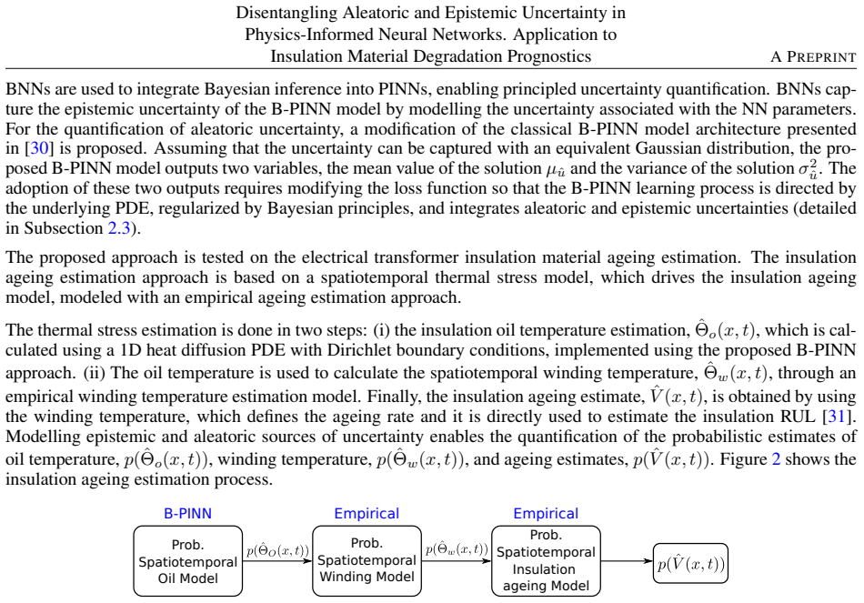
- The full pipeline—oil temperature, winding temperature, ageing acceleration, loss of life—propagates the predictive temperature distribution into a distribution over insulation ageing, which is the quantity maintenance decisions actually need.
Reading between the lines
- Inference: the same dual-output heteroscedastic treatment likely transfers to other degradation prognostics governed by parabolic heat equations, such as battery thermal runaway or bearing heat diffusion, where noise is also load-dependent.
- Inference: the reported 'true' temperature is a finite-element simulation, not a full set of internal sensor measurements; how much of the comparative advantage holds in the physical transformer is an open question the paper's setup cannot settle.
- Inference: the learned aleatoric variance could be reused as an acquisition function, sampling more collocation points where variance is high and CRPS is worst, which the paper does not test.
- Inference: since epistemic uncertainty stayed small while aleatoric dominated, a cheaper surrogate that only models heteroscedastic noise might capture most of the practical benefit; the paper does not test this.
Editorial analysis
A structured set of objections, weighed in public.
Referee Report
Summary. This paper proposes a heteroscedastic Bayesian physics-informed neural network (B-PINN) that outputs both a predictive mean and an input-dependent variance for a 1D heat-diffusion model of transformer oil temperature, and couples it with empirical winding-temperature and IEC ageing models to produce probabilistic insulation-ageing estimates. Epistemic uncertainty is represented by variational inference over network weights; aleatoric uncertainty is modeled through a Gaussian likelihood with a learned variance. The method is compared with vanilla PINNs, dropout PINNs, and a homoscedastic B-PINN on a floating-solar-plant transformer case study, using a finite-element solution as the reference. The authors claim improved predictive accuracy and better-calibrated uncertainty estimates, and they report a sensitivity study of initial, boundary, and residual sampling strategies.
Significance. If the headline results held, the paper would provide a practically motivated demonstration that heteroscedastic Bayesian PINNs can disentangle aleatoric and epistemic uncertainty in a PHM application. The strengths are the realistic transformer case study, the comparison with several baselines, and the sensitivity analysis of sampling strategies. However, the central methodological novelty is largely a standard combination of heteroscedastic BNN regression with PINN residuals, and the empirical support is weakened by an underspecified residual likelihood, overlapping confidence intervals, and an evaluation that is effectively interpolation against a simulation rather than forecasting against independent field data. No code or data are provided, which further limits reproducibility. The contribution is therefore better characterized as an application study whose headline claims require substantial revision.
major comments (3)
- [Section 2.4, Eq. (21)] The training objective for the heteroscedastic B-PINN is not well-defined. Eq. (20) defines NLL_hetero(x,t;θ) for a point with an observed solution value u. Eq. (21) reuses this NLL for residual points as λ_r NLL_hetero^(r), but no formula for NLL_hetero^(r) is given. At residual collocation points there is no observed u; the quantity being minimized is r(x,t;θ)=L[u_θ]-f, and one cannot simply take σ^2_hat u(x,t;θ), the network's output variance, as the variance of r. The homoscedastic formulation in Eq. (14) used a fixed σ_f for residual points, but the heteroscedastic extension silently changes this. Algorithm 2, the only training algorithm supplied, still refers to Eq. (15) and the homoscedastic residual likelihood, not to Eq. (21). Since the reported accuracy and calibration results are obtained by minimizing this objective, the central claim is not internally supported until the res
- [Tables 2 and 3] The headline claim of better-calibrated uncertainty estimates is not supported by the reported statistics. At t=6h, the heteroscedastic B-PINN NLL is 1.61±1.43, worse than the homoscedastic 0.49±0.33. Total NLL values overlap within standard deviations (1.75±0.19 vs 1.98±0.73). Miscalibration areas also overlap (0.1956±0.1616 vs 0.2135±0.0591). With only five runs, these differences are not statistically significant. The text acknowledges the t=6h exception but still claims an overall 11.6% NLL improvement and marginally better calibration; the evidence presented does not establish superiority. The authors should either provide significance tests, confidence intervals, or substantially weaken the comparative claims.
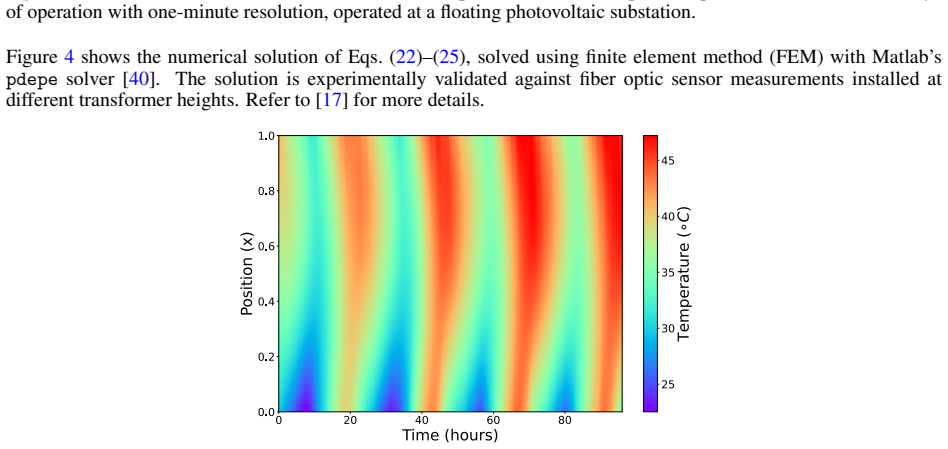
- [Sections 3.1–3.2 and Appendix A] The evaluation does not support the 'prognostics' and 'generalization' claims. The FEM solution of Eqs. (22)–(25) is used both to define the initial and boundary conditions for training (Fig. 4, §3.1) and as the reference for computing ageing errors (Fig. 9). The 'prediction instants' reported in Table 2 (t=0, 3, 6, 18, 25, 50 h) all lie inside the four-day training window shown in Fig. 3, so the experiments measure interpolation to simulated data, not forecasting to unseen future conditions. The ageing error in Fig. 9 is computed against the same FEM model, not against independent field measurements. The abstract's 'generalization' and 'prognostics' claims therefore need to be substantially qualified, or the evaluation needs a held-out temporal split and an independent validation data source.
minor comments (4)
- [Section 2.2, Eq. (11)] Typo: 'equivalenty implemented' should be 'equivalently implemented'. Also, the notation for variance is inconsistent: Eq. (20) uses σ^2_hat u, while Eq. (35) in Appendix B uses σ(x_i)^2; please unify.
- [Table 5] The row 'Loss Function - -ELBO' is confusing for the d-PINN model, since the d-PINN loss is defined via Eq. (35), not the ELBO. The table should state the actual loss used for each configuration.
- [Figure 10] The markers and error annotations in the sensitivity figure are difficult to read in print. Please enlarge the figure, use distinct markers, and report the numerical values in a table.
- [Abstract and Section 1] The abstract says the framework is 'validated with a finite-element thermal model and field measurements from a solar power plant', but the paper directly validates only the FEM model with field measurements (via ref. [17]); the B-PINN output is compared with the FEM simulation, not with the field measurements. Please clarify this distinction to avoid overstating the validation.
Circularity Check
Heteroscedastic residual loss is self-referential and headline 'prediction' metrics are in-sample, so the claimed improvements are not independently established.
-
self definitional
[Section 2.4, Eqs. (20)-(21); residual definition Eq. (6)]
"NLL_hetero(x, t; θ) = 1/2 log(2π σ^2_û(x,t;θ)) + (u − µ_û(x,t;θ))^2/(2σ^2_û(x,t;θ)) ... where u is the solution or ground truth ... each NLL^(.)_hetero(θ(k)) term is the sum over the corresponding initial condition, boundary condition and residual points of Eq. (20)."
Residual points have no observed ground-truth u: the object at those points is r(x,t;θ)=L[û]−f. Applying Eq. (20) at residual points therefore forces the residual likelihood to use the network's solution-variance output σ^2_û as the variance of r. For fixed r, minimizing the resulting term with respect to σ^2_û gives σ^2_û = r², so the physics residual can be made nearly costless by inflating the predicted variance. The 'aleatoric variance' that is later reported as the data-noise component is the same variable that controls the physics penalty; the physics constraint and the fitted uncertainty output are defined in terms of each other, not independently anchored.
-
fitted input called prediction
[Section 3.1 training setup and Table 2 prediction instants]
"Figure 3 shows the available minutely sampled time series ... with a total of 5760 samples over 4 days of operation. ... All B-PINN models are trained for 15000 epochs, with early stopping ... Table 2 reports the probabilistic performance metrics ... across different prediction instants ... Instant [h] 0 ... 50."
No train/test split is described: the model is trained on the full 4-day domain, and every reported 'prediction instant' (0, 3, 6, 18, 25, 50 h) lies inside that domain. The RMSE, CRPS, and NLL values in Table 2 are therefore in-sample fit errors, not forecasts from a cutoff time. The headline 57.3% RMSE improvement over the vanilla PINN is a comparison of training-fit quality on the same spatiotemporal window, so the claimed predictive advantage is statistically forced by the training configuration rather than demonstrated on held-out future data.
full rationale
The paper is not wholly self-referential: it uses an external FEM solver (Matlab pdepe), operational field measurements, and standard IEC ageing equations, and the law-of-total-variance decomposition in Eq. (19) is a standard identity. However, the central claimed improvement of the heteroscedastic B-PINN has two load-bearing reductions. First, Eq. (21) reuses the heteroscedastic NLL of Eq. (20) for residual points, where no ground-truth u exists; the only coherent instantiation makes the residual variance equal to the network's learned solution variance, so the physics residual can be satisfied by increasing the output variance rather than by reducing r. This makes the 'aleatoric uncertainty' and the residual penalty the same fitted variable, and Algorithm 2 still refers to the earlier homoscedastic objective, so the actual training objective is both self-referential and unverified. Second, the evaluation instants all fall inside the training time window and no temporal holdout is described, so the reported RMSE/CRPS/NLL gains are in-sample fit metrics, not prognostics predictions. The hyperparameter and baseline configurations inherited from the authors' prior work ([17], [30], [15]) add a self-citation flavor, but the main circularity is the self-referential residual likelihood and the in-sample prediction evaluation. Score 6: partial circularity with the central claim reducing by construction to fitted quantities.
Assumptions & free parameters
free parameters (5)
- Loss weights λ0, λb, λr =
λ0=1, λb=1, λr=1e-4
- Homoscedastic noise std σ_i, σ_r =
0.01, 0.01
- d-PINN dropout rate ρ =
0.1
- Network architecture =
2 layers × 50 neurons
- Optimizer hyperparameters =
Adam lr=0.01, batch=16, 15000 epochs
assumptions (7)
- domain assumption 1D heat diffusion PDE (Eq. 22) with radiative heat transfer and no convection
- domain assumption Dirichlet boundary conditions (Eq. 25): ΘO(0,t)=ΘA(t), ΘO(H,t)=ΘTO(t)
- domain assumption IEC 60076-7 empirical winding/HST model (Eqs. 26-29)
- domain assumption Ageing acceleration model V=2^((ΘH−98)/6) (Eq. 31)
- ad hoc to paper Gaussian likelihood for aleatoric uncertainty (Eqs. 16, 20)
- standard math Gaussian variational posterior and reparameterization trick
- standard math Law of total variance decomposition (Eq. 19)
Cite this review
Pith. "Pith review of Disentangling Aleatoric and Epistemic Uncertainty in Physics-Informed Neural Networks. Application to Insulation Material Degradation Prognostics." pith.science (2026). https://pith.science/paper/FVGGJ2FB
@misc{pith2026260103673,
  author       = {Pith},
  title        = {Pith review of: Disentangling Aleatoric and Epistemic Uncertainty in Physics-Informed Neural Networks. Application to Insulation Material Degradation Prognostics},
  year         = {2026},
  howpublished = {\url{https://pith.science/paper/FVGGJ2FB}},
  note         = {Machine review of arXiv:2601.03673}
}
read the original abstract
Physics-Informed Neural Networks (PINNs) provide a framework for integrating physical laws with data. However, their application to Prognostics and Health Management (PHM) remains constrained by the limited uncertainty quantification (UQ) capabilities. Most existing PINN-based prognostics approaches are deterministic or account only for epistemic uncertainty, limiting their suitability for risk-aware decision-making. This work introduces a heteroscedastic Bayesian Physics-Informed Neural Network (B-PINN) framework that jointly models epistemic and aleatoric uncertainty, yielding full predictive posteriors for spatiotemporal insulation material ageing estimation. The approach integrates Bayesian Neural Networks (BNNs) with physics-based residual enforcement and prior distributions, enabling probabilistic inference within a physics-informed learning architecture. The framework is evaluated on transformer insulation ageing application, validated with a finite-element thermal model and field measurements from a solar power plant, and benchmarked against deterministic PINNs, dropout-based PINNs (d-PINNs), and alternative B-PINN variants. Results show that the proposed B-PINN provides improved predictive accuracy and better-calibrated uncertainty estimates than competing approaches. A systematic sensitivity study further analyzes the impact of boundary-condition, initial-condition, and residual sampling strategies on accuracy, calibration, and generalization, and the influence of measurement noise on aleatoric uncertainty. Overall, the findings highlight the capability of Bayesian physics-informed learning to support uncertainty-aware prognostics and informed decision-making in transformer asset management by tracking aleatoric and epistemic sources of uncertainty.
Figures


Figures from the paper (10 more)


Reference graph
Works this paper leans on
-
[1]
G. J. Vachtsevanos, F. Lewis, M. Roemer, A. Hess, B. Wu,Intelligent fault diagnosis and prognosis for engi- neering systems, volume 456, Wiley Online Library,2006
2006
-
[2]
Kordestani, M
M. Kordestani, M. Saif, M. E. Orchard, R. Razavi-Far, K. Khorasani,IEEE Transactions on Reliability2021, 70, 2 728
-
[3]
G. E. Karniadakis, I. G. Kevrekidis, L. Lu, P. Perdikaris, S. Wang, L. Yang,Nature Reviews Physics2021,3, 6 422
-
[5]
Kovachki, Z
N. Kovachki, Z. Li, B. Liu, K. Azizzadenesheli, K. Bhattacharya, A. Stuart, A. Anandkumar,J. Mach. Learn. Res.2023,24, 1
2023
-
[6]
Z. Li, H. Zheng, N. Kovachki, D. Jin, H. Chen, B. Liu, K. Azizzadenesheli, A. Anandkumar,ACM / IMS J. Data Sci.2024,1, 3
2024
-
[7]
Z. Liu, Y . Wang, S. Vaidya, F. Ruehle, J. Halverson, M. Solja ˇci´c, T. Y . Hou, M. Tegmark, InInternational Conference on Learning Representations (ICLR).2025
2025
-
[8]
J. D. Toscano, V . Oommen, A. J. Varghese, Z. Zou, N. A. Daryakenari, C. Wu, G. E. Karniadakis,Mach. Learn. Comput. Sci. Eng.2025,1, 15
2025
-
[9]
J. I. Aizpurua, V . M. Catterson, InAnnual Conference of the PHM Society, volume 7.2015
2015
Show all 45 references
-
[10]
J. Guo, Z. Li, M. Li,IEEE Transactions on Reliability2020,69, 3 1110
-
[11]
Zio,Reliability Engineering & System Safety2022,218108119
E. Zio,Reliability Engineering & System Safety2022,218108119
-
[12]
Arias Chao, C
M. Arias Chao, C. Kulkarni, K. Goebel, O. Fink,Reliability Engineering & System Safety2022,217107961
-
[13]
Daigle, I
M. Daigle, I. Roychoudhury, A. Bregon, InAnnual Conference of the PHM Society, volume 7.2015. 17 Disentangling Aleatoric and Epistemic Uncertainty in Physics-Informed Neural Networks. Application to Insulation Material Degradation PrognosticsA PREPRINT
2015
-
[14]
J. I. Aizpurua, I. Ramirez, I. Lasa, L. d. Rio, A. Ortiz, B. G. Stewart,IEEE Trans. Pow. Del.2023,38, 1 599
2023
-
[15]
Alcibar, J
J. Alcibar, J. I. Aizpurua, E. Zugasti, O. Pe ˜nagarikano,Engineering Applications of Artificial Intelligence2025, 146110246
-
[16]
F. Wang, Z. Zhai, Z. Zhao, Y . Di, X. Chen,Nature Communications2024,15, 1 4332
-
[17]
Ramirez, J
I. Ramirez, J. Pino, D. Pardo, M. Sanz, L. del Rio, A. Ortiz, K. Morozovska, J. I. Aizpurua,Engineering Applications of Artificial Intelligence2025,139109556
-
[18]
Sankararaman,Mechanical Systems and Signal Processing2015,52228
S. Sankararaman,Mechanical Systems and Signal Processing2015,52228
-
[19]
Salinas-Camus, K
M. Salinas-Camus, K. Goebel, N. Eleftheroglou,Mechanical Systems and Signal Processing2025,237113015
-
[20]
Linka, A
K. Linka, A. Sch ¨afer, X. Meng, Z. Zou, G. E. Karniadakis, E. Kuhl,Computer Methods in Applied Mechanics and Engineering2022,402115346
-
[21]
J. Li, X. Long, X. Deng, W. Jiang, K. Zhou, C. Jiang, X. Zhang,Reliability Engineering & System Safety2024, 245109963
-
[22]
A. S. Nair, B. Jacob, A. A. Howard, J. Drgona, P. Stinis, E-pinns: Epistemic physics-informed neural networks, 2025
2025
-
[23]
Podina, M
L. Podina, M. T. Rad, M. Kohandel, InICLR 2024 Workshop on AI4Differential Equations In Science.2024
2024
-
[24]
Zhang, L
D. Zhang, L. Lu, L. Guo, G. E. Karniadakis,Journal of Computational Physics2019,397108850
-
[25]
Jiang, X
X. Jiang, X. Wang, Z. Wen, E. Li, H. Wang,International Communications in Heat and Mass Transfer2023, 147106940
-
[26]
Z. Zou, Z. Wang, G. E. Karniadakis,arXiv preprint arXiv:2503.063202025
-
[27]
H ¨ullermeier, W
E. H ¨ullermeier, W. Waegeman,Machine learning2021,110, 3 457
-
[28]
Fern ´andez, J
J. Fern ´andez, J. Chiach´ıo, M. Chiach´ıo, J. Barros, M. Corbetta,Engineering Applications of Artificial Intelligence 2023,119105790
2023
-
[29]
R. G. Nascimento, F. A. Viana, M. Corbetta, C. S. Kulkarni,Scientific Reports2023,13, 1 13856
-
[30]
Ramirez, J
I. Ramirez, J. Alcibar, J. Pino, M. Sanz, D. Pardo, J. I. Aizpurua, InAnnual Conference of the PHM Society, volume 17.2025
2025
-
[31]
Aizpurua, B
J. Aizpurua, B. Stewart, S. McArthur, M. Penalba, M. Barrenetxea, E. Muxika, J. Ringwood,Reliability Engi- neering & System Safety2022,226108676
-
[32]
Raissi, P
M. Raissi, P. Perdikaris, G. Karniadakis,Journal of Computational Physics2019,378686
-
[33]
L. G. Wright, T. Onodera, M. M. Stein, T. Wang, D. T. Schachter, Z. Hu, P. L. McMahon,Nature2022,601, 7894 549
-
[34]
S. J. Anagnostopoulos, J. D. Toscano, N. Stergiopulos, G. E. Karniadakis,Computer Methods in Applied Me- chanics and Engineering2024,421116805
-
[35]
Fortuin, A
V . Fortuin, A. Garriga-Alonso, M. van der Wilk, L. Aitchison,Software Impacts2021,9100079
-
[36]
Kendall, Y
A. Kendall, Y . Gal, In I. Guyon, U. V . Luxburg, S. Bengio, H. Wallach, R. Fergus, S. Vishwanathan, R. Garnett, editors,Advances in Neural Information Processing Systems, volume 30. Curran Associates, Inc.,20171–11
-
[37]
M. E. Orchard, G. J. Vachtsevanos,Transactions of the Institute of Measurement and Control2009,31, 3-4 221
-
[38]
H ¨ullermeier, W
E. H ¨ullermeier, W. Waegeman,Machine Learning2021,110, 3 457
-
[39]
Depeweg, J.-M
S. Depeweg, J.-M. Hernandez-Lobato, F. Doshi-Velez, S. Udluft, In J. Dy, A. Krause, editors,Proceedings of the 35th International Conference on Machine Learning, volume 80 ofProceedings of Machine Learning Research. PMLR,20181184–1193
-
[40]
The MathWorks, Inc.,PDEPE Toolbox, Natick, Massachusetts, USA,2023, URLhttps://mathworks.com/
2023
-
[41]
International Electrotechnical Commission,IEC 60076-72018
-
[42]
Y . Gal, Z. Ghahramani, In M. F. Balcan, K. Q. Weinberger, editors,Proceedings of The 33rd International Conference on Machine Learning, volume 48 ofProceedings of Machine Learning Research. PMLR, New York, New York, USA,20161050–1059
-
[43]
K. P. Murphy,Machine learning: a probabilistic perspective, MIT press,2012
2012
-
[44]
C. M. Bishop, N. M. Nasrabadi,Pattern recognition and machine learning, volume 4, Springer,2006
2006
-
[45]
M. Zamo, P. Naveau,Mathematical Geosciences2018,50, 2 209
-
[46]
Gneiting, A
T. Gneiting, A. E. Raftery, A. H. Westveld, T. Goldman,Monthly Weather Review2005,133, 5 1098. 18 Disentangling Aleatoric and Epistemic Uncertainty in Physics-Informed Neural Networks. Application to Insulation Material Degradation PrognosticsA PREPRINT A Transformer Thermal M...
Reviewed August 3, 2026 · model on record in the stance chip above.
Discussion (0). Continue with ORCID to comment.