REVIEW 5 major objections 5 minor 34 references
Binary Tree Option Pricing Under Market Microstructure Effects: A Random Forest Approach
T0 review · 5 major / 5 minor · reviewed 2026-08-06 · deepseek-v4-flash
Pith's one-line read A Random Forest trained on minute-level SPY data supplies path-dependent probabilities to a binomial tree, which prices a 30-day call at $15.41, 13.79% below Black-Scholes.
desk verdict Honest proof of concept whose headline pricing result is an artifact of an unvalidated time-scaling step, and whose MMM 'optimization' is vacuous. read the letter →
The pith
A machine-rendered reading of the paper's core claim, the machinery that carries it, and where it could break.
The reading
What carries the argument
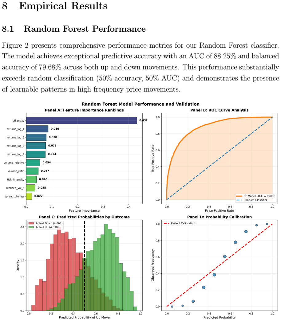
The central object is the microstructure-enhanced binary tree (Definition 1), a binomial tree whose nodes carry not just price $S_i$ but a microstructure state $s_i = (S_i, m_i)$; at each node the up/down factors $u(s)$, $d(s)$ and the up probability are state-dependent. A Random Forest with a 17-dimensional feature map $\phi(s)$—lagged returns, spread proxies, volume, realized volatility, order flow imbalance, and time features—produces the physical up-probability $p_{\mathrm{RF}}(s)$. The no-arbitrage mechanism is the minimal martingale measure: $p^{*}(s) = (e^{r\Delta t} - d(s))/(u(s)-d(s))$, which keeps the discounted price a martingale while staying close to the empirical probabilities. The third mechanical piece is the square-root-of-time rescaling, factor $\sqrt{807.8}$, that converts minute-level conditional moments to three-day tree steps, along with the implementation's reduction of the 17 features to 20 probability-based states.
What would settle it
Compute the same 30-day call with the tree built from minute-level steps (no $\sqrt{807.8}$ rescaling) using the Random Forest probabilities; the paper's own unscaled result of $0.38 shows how much the price depends on that scalar, and a three-day-step tree with moments estimated directly from three-day returns would settle whether $15.41 survives without the rescaling.
Extended reading notes
Core claim
The paper's central claim is that the physical probability of an up-move in a binary tree can be learned directly from high-frequency data and then minimally adjusted to a risk-neutral probability, preserving no-arbitrage while carrying microstructure information into the option price. State-dependent up and down factors $u(s)$ and $d(s)$ are calibrated to conditional moments in each of 20 market states, and the adjustment is the minimal martingale measure $p^{*}(s) = (e^{r\Delta t} - d(s))/(u(s)-d(s))$, the probability that makes the discounted price process a martingale while remaining as close as possible to the Random Forest's physical estimate. The authors report that the resulting risk-neutral probabilities differ from the physical ones by an average of 21.7%, and that state-dependent implied volatilities range from 16.2% to 70.7% annualized. Applied to a 30-day at-the-money SPY call with 10 three-day tree steps, the method gives $15.41 versus a Black-Scholes price of $17.87, a difference the paper attributes to microstructure effects that classical models miss.
Load-bearing premise
The load-bearing premise is that probabilities and variances estimated from one-minute price moves remain valid after being rescaled by the square root of time to represent three-day tree steps; if intraday states do not persist across days, the reported $15.41 price is an artifact of that scaling.
Editorial extensions
If this is right
- If the framework is right, short-dated at-the-money option prices can differ from Black-Scholes by more than 10% purely because of microstructure, which means market makers and risk managers should treat the classical model as a biased benchmark for such options.
- Order flow imbalance carries pricing information for short-term options, so flow data belongs in the feature set of any empirical option-pricing model.
- Risk premiums are state-dependent: because physical and risk-neutral probabilities differ by 21.7% on average and vary across the 20 states, a single constant risk-neutral probability understates the structure of short-term risk compensation.
- The method's current limits are computational: with exponential node growth and three-day time steps, the reported evidence covers only short maturities, so the size of the microstructure effect on longer-dated options is not yet established.
Reading between the lines
- Beyond the paper: the 13.79% gap is a statement about this model's chosen risk-neutral measure, not a direct estimate of market mispricing; a natural extension is to compare the tree's prices for multiple strikes and maturities against observed SPY option quotes to see whether the gap persists.
- Beyond the paper: because the implementation collapses the 17-dimensional feature space to 20 probability bins, the reported price likely understates the model's sensitivity to microstructure; a finer state resolution could move the price in either direction.
- Beyond the paper: the square-root-of-time rescaling of minute-level moments to three-day steps is the assumption most likely to break; re-estimating the same 20 states from multi-day returns would provide a direct test of whether the $15.41 price is driven by microstructure or by the rescaling.
- Beyond the paper: the state-dependent volatility clustering (16.2% to 70.7% annualized) points to a concrete risk-management extension—value-at-risk and hedge ratios that condition on the current microstructure state—that the paper does not test.
Signed reviews
Editorial analysis
A structured set of objections, weighed in public.
Referee Report
Summary. The paper proposes a binomial tree option pricing model in which transition probabilities are learned by a Random Forest classifier from minute-level SPY data, and state-dependent up/down factors are calibrated to conditional return moments. No-arbitrage is imposed through a claimed 'minimal martingale measure' adjustment, and the resulting 10-step tree prices a 30-day ATM SPY call at $15.41, 13.79% below the Black-Scholes price of $17.87. The paper also reports an AUC of 88.25% for one-minute direction prediction and identifies order flow imbalance as the dominant feature. The authors repeatedly acknowledge severe computational and implementation limitations, including a prior time-scaling error that produced a $0.38 price.
Significance. If the central claims were established, the paper would present a meaningful step toward integrating machine-learning-based microstructure information into arbitrage-free option pricing. The empirical observation that order flow imbalance dominates Random Forest feature importance for minute-level SPY direction is potentially interesting, and the paper is unusually transparent about its own limitations and implementation failures. However, the headline pricing result is not supported: the 'minimal martingale measure' step is mathematically vacuous, the square-root-of-time scaling that produces the $15.41 price is unvalidated, and the implemented tree discards the very path-dependence that motivates the framework. The paper's significance is therefore not yet demonstrated, and the current evidence does not establish a robust data-driven alternative to classical pricing.
major comments (5)
- [Section 4.2, Eqs. (7)-(8)] The constrained KL divergence minimization stated in Eq. (7) does not lead to Eq. (8). For fixed u(s) and d(s), the KL minimizer satisfies p*/(1-p*) = [p_RF(s)/(1-p_RF(s))] exp(-λ(u(s)-d(s))) with λ chosen to meet the constraint; this equals the martingale probability (e^{rΔt}-d(s))/(u(s)-d(s)) only for a special choice of p_RF(s). Eq. (8) is simply the solution of the no-arbitrage equation (6) for p*, so the 'Minimal Martingale Measure' language and the 'optimal balance' claim are not justified. This also explains why Section 8.4 reports optimization costs of 0.0: no optimization over measures was actually performed.
- [Section 8.4 and Table 4] The square-root-of-time scaling factor √807.8 converts per-minute movement factors to 3-day tree steps. This assumes that the market state identified at one minute persists for approximately 808 minutes and that conditional returns within that state are iid, so that the conditional mean scales as n·μ(s) and the conditional variance as n·σ²(s). No evidence is provided for either assumption, and the paper does not state how the drift in Eq. (11) is scaled separately from the volatility. The reported $15.41 price and the 13.79% gap versus Black-Scholes are therefore not identified as a microstructure effect; they depend crucially on the unvalidated scaling rule. Direct validation against empirical 3-day conditional return moments, or a multi-day out-of-sample exercise, is required before the headline deviation can be accepted.
- [Section 8.5 and Table 4] The implemented tree uses 20 states formed by binning Random Forest probability values and maps each node to the nearest state solely on p_RF, discarding the 17-dimensional feature vector, as acknowledged in Section 9.4.2. Consequently the 'path-dependent transition probabilities' claimed in the abstract are not realized in the pricing exercise; the tree is state-dependent only in a single scalar. Moreover, with 10 steps of 3 days each, the model cannot capture minute-level microstructure dynamics, so the pricing result does not support the conclusion that microstructure effects matter for option values.
- [Section 8.1 and Table 2] The cross-validation design is not specified. If the reported AUC of 0.8825 comes from random K-fold splits of minute-level series, temporal leakage (training on future data relative to validation) will inflate the metric. The paper should use walk-forward or blocked time-series validation. In addition, the 'order flow imbalance' feature is not defined precisely; the data section should state how signed volume is obtained from the available OHLCV and tick data.
- [Sections 5.3 and 9.4.3] The optimization in Eq. (14) is never actually carried out; reporting that 'all 20 market states converged immediately with optimization costs of 0.0' means the weights w1 and w2 play no role in the results. This is inconsistent with the average absolute difference of 0.217 between p_RF and p_MMM reported in Table 3, since the KL divergence term in Eq. (14) would be strictly positive. The paper should either implement the stated optimization or explicitly state that no-arbitrage is enforced solely by Eq. (8).
minor comments (5)
- [Throughout] The manuscript contains many typographical and formatting issues, including 'Ivas,cu' in the literature review, 'HilliardandSchwartz' without spaces, inconsistent capitalization of O'Hara, and a misspelling of Møller in the Schweizer reference.
- [Algorithm 1] Line 8 instructs the reader to 'solve for u(s), d(s) that match moments and ensure no-arbitrage', but this system is generally overdetermined; the text should clarify the sequential procedure actually used.
- [Section 7.2] The order flow imbalance proxy should be fully defined, including the sign convention and the construction of signed volume from the available data; Figure 1, Panel D currently refers to a distribution of an undefined variable.
- [Table 4] The entry 'Scaling Factor Applied √807.8' does not state whether the drift term in Eq. (11) is also scaled linearly in time; please specify the full transformation of both factors.
- [Section 8.6] The claim that feature importance is stable across sub-periods (correlation > 0.95) is reported without showing how the sub-periods are defined; please provide details or a supplementary figure.
Circularity Check
The no-arbitrage 'calibration success' is definitional: Eq. (8) forces the constraint in Eq. (6), so zero optimization cost is a tautology. The 13.79% option-price gap itself is not circular, but the paper's claim that MMM calibration empirically succeeds reduces to its own definition.
-
self definitional
[Section 4.2, Eq. (8); Section 8.4]
"This leads to a state-dependent risk-neutral probability: pMMM(s) = (e^{rΔt} − d(s))/(u(s) − d(s)) (8) ... All 20 market states converged immediately with optimization costs of 0.0, indicating that the initial moment-matching procedure already approximated no-arbitrage conditions within computational tolerance."
Equation (8) is obtained by solving the no-arbitrage constraint Eq. (6), p*(s)u(s)+(1−p*(s))d(s)=e^{rΔt}, for p*. Therefore the constraint holds identically for every state, for any fitted u(s) and d(s). The reported 'convergence' with zero optimization cost is not an empirical finding about the data or about moment matching; it is a mathematical identity. The paper presents this as evidence that the Minimal Martingale Measure calibration succeeded, but the success is built into the formula by construction.
full rationale
The central pricing output, the $15.41 call price and its 13.79% deviation from Black-Scholes, is not itself circular: it is produced by fitting state-dependent up/down factors to empirical conditional moments, applying the sqrt(807.8) time-scaling, and running backward induction. That chain could have produced a different number and is externally benchmarked against Black-Scholes. The circularity is confined to the paper's no-arbitrage validation narrative: Section 8.4 reports zero-cost MMM convergence as a discovery, but Eq. (8) defines pMMM exactly as the solution of the no-arbitrage equation, so the outcome is guaranteed. Relatedly, the MMM framing in Eqs. (7)-(8) is vacuous as an optimization because the no-arbitrage constraint alone fixes p* for given u(s), d(s); the KL divergence plays no selective role. That is more a relabeling/correctness concern than a circular step. The self-citations (Deep et al., Lauria et al.) are not load-bearing for the pricing result, which rests on the paper's own RF fit and factor calibration. The unvalidated sqrt-of-time aggregation of one-minute moments to 3-day steps is a serious fragility, but it is an assumption about persistence and scaling, not a circular derivation. Overall, partial circularity: the no-arbitrage 'prediction' reduces by definition, while the headline option-price gap retains independent empirical content. Score 6 reflects that partial reduction rather than the 8-10 range, which would require the whole price derivation to be forced by definition or by a self-citation chain.
Assumptions & free parameters
free parameters (5)
- Time scaling factor sqrt(807.8) =
sqrt(807.8)
- Number of market states =
20
- Random Forest hyperparameters =
Not fully reported; sensitivity described for 100-500 trees
- Feature window lengths =
k=5 lags, 5-minute windows
- Optimization weights w1, w2 in Eq. (14) =
Not reported
assumptions (5)
- domain assumption Random Forest output probabilities are well-calibrated physical probabilities of up-moves.
- domain assumption Minimal martingale measure is the appropriate pricing measure in this incomplete market.
- ad hoc to paper Square-root-of-time scaling of minute-level movement factors to 3-day steps is valid.
- ad hoc to paper A 20-state aggregation based only on Random Forest probability values is sufficient to capture path-dependent microstructure.
- domain assumption The six months of January to June 2025 SPY data are representative for pricing a 30-day option.
Cite this review
Pith. "Pith review of Binary Tree Option Pricing Under Market Microstructure Effects: A Random Forest Approach." pith.science (2026). https://pith.science/paper/GNU6R7S4
@misc{pith2026250716701,
  author       = {Pith},
  title        = {Pith review of: Binary Tree Option Pricing Under Market Microstructure Effects: A Random Forest Approach},
  year         = {2026},
  howpublished = {\url{https://pith.science/paper/GNU6R7S4}},
  note         = {Machine review of arXiv:2507.16701}
}
read the original abstract
We propose a machine learning-based extension of the classical binomial option pricing model that incorporates key market microstructure effects. Traditional models assume frictionless markets, overlooking empirical features such as bid-ask spreads, discrete price movements, and serial return correlations. Our framework augments the binomial tree with path-dependent transition probabilities estimated via Random Forest classifiers trained on high-frequency market data. This approach preserves no-arbitrage conditions while embedding real-world trading dynamics into the pricing model. Using 46,655 minute-level observations of SPY from January to June 2025, we achieve an AUC of 88.25% in forecasting one-step price movements. Order flow imbalance is identified as the most influential predictor, contributing 43.2% to feature importance. After resolving time-scaling inconsistencies in tree construction, our model yields option prices that deviate by 13.79% from Black-Scholes benchmarks, highlighting the impact of microstructure on fair value estimation. While computational limitations restrict the model to short-term derivatives, our results offer a robust, data-driven alternative to classical pricing methods grounded in empirical market behavior.
Figures


Reference graph
Works this paper leans on
-
[1]
Bahsoun, W., Góra, P., Mayoral, S., and Morales, M. (2007). Random dynamics and finance: Constructing implied binomial trees from a predetermined stationary density. Applied Stochastic Models in Business and Industry, 23(3):181–212. 30
work page 2007
-
[2]
Bandi, F. M., Russell, J. R., and Zhu, Y. (2008). Using high-frequency data in dynamic portfolio choice. Econometric Reviews, 27(1-3):163–198
work page 2008
-
[3]
Black, F. and Scholes, M. (1973). The pricing of options and corporate liabilities.Journal of political economy, 81(3):637–654
work page 1973
-
[4]
Boyle, P. P. (1988). A lattice framework for option pricing with two state variables. Journal of financial and quantitative analysis, 23(1):1–12
work page 1988
-
[5]
Boyle, P. P. and Vorst, T. (1992). Option replication in discrete time with transaction costs. The Journal of Finance, 47(1):271–293
work page 1992
-
[6]
Broadie, M. and Detemple, J. (1996). American option valuation: new bounds, approx- imations, and a comparison of existing methods. The Review of Financial Studies, 9(4):1211–1250
work page 1996
-
[7]
Brogaard, J., Hendershott, T., and Riordan, R. (2014). High-frequency trading and price discovery. The Review of Financial Studies, 27(8):2267–2306
work page 2014
-
[8]
Christoffersen, P., Fournier, M., and Jacobs, K. (2018). The factor structure in equity options. The Review of Financial Studies, 31(2):595–637
work page 2018
Show all 34 references
-
[9]
and Tankov, P
Cont, R. and Tankov, P. (2003).Financial modelling with jump processes. Chapman and Hall/CRC
2003
-
[10]
C., Ross, S
Cox, J. C., Ross, S. A., and Rubinstein, M. (1979). Option pricing: A simplified approach. Journal of financial Economics, 7(3):229–263
1979
-
[11]
Deep, A. (2023). A multifactor analysis model for stock market prediction.International Journal of Computer Science and Telecommunications, 14(1)
2023
-
[12]
Deep, A., Shirvani, A., Monico, C., Rachev, S., and Fabozzi, F. (2025). Risk-adjusted performance of random forest models in high-frequency trading.Journal of Risk and Financial Management, 18(3):142
2025
-
[13]
Deep, A. T. (2024). Advanced financial market forecasting: integrating monte carlo simulations with ensemble machine learning models
2024
-
[14]
and Schachermayer, W
Delbaen, F. and Schachermayer, W. (2006). A general version of the fundamental theorem of asset pricing (1994). InThe Mathematics of Arbitrage, pages 149–205. Springer
2006
-
[15]
Easley, D., O’hara, M., and Srinivas, P. S. (1998). Option volume and stock prices: Evidence on where informed traders trade.The Journal of Finance, 53(2):431–465
1998
-
[16]
and Sirignano, J
Fan, L. and Sirignano, J. (2024). Machine learning methods for pricing financial deriva- tives. arXiv preprint arXiv:2406.00459. 31
2024 arXiv
-
[17]
Frittelli, M. (2000). The minimal entropy martingale measure and the valuation problem in incomplete markets.Mathematical finance, 10(1):39–52
2000
-
[18]
Gu, S., Kelly, B., and Xiu, D. (2020). Empirical asset pricing via machine learning.The Review of Financial Studies, 33(5):2223–2273
2020
-
[19]
Harrison, J. M. and Kreps, D. M. (1979). Martingales and arbitrage in multiperiod securities markets. Journal of Economic Theory, 20(3):381–408
1979
-
[20]
Martingalesandstochasticintegralsinthetheory of continuous trading.Stochastic Processes and their Applications, 11(3):215–260
Harrison, J.M.andPliska, S.R.(1981). Martingalesandstochasticintegralsinthetheory of continuous trading.Stochastic Processes and their Applications, 11(3):215–260
1981
-
[21]
and Zhu, S.-P
He, X.-J. and Zhu, S.-P. (2016). Pricing european options with stochastic volatility under the minimal entropy martingale measure.European Journal of Applied Mathematics, 27(2):233–247
2016
-
[22]
Hilliard, J. E. and Schwartz, A. (2005). Pricing european and american derivatives un- der a jump-diffusion process: A bivariate tree approach. Journal of Financial and Quantitative Analysis, 40(3):671–691
2005
-
[23]
Horvath, B., Muguruza, A., and Tomas, M. (2021). Deep learning volatility: a deep neural network perspective on pricing and calibration in (rough) volatility models. Quantitative Finance, 21(1):11–27
2021
-
[24]
Hull, J. C. and White, A. D. (1993). Efficient procedures for valuing european and american path-dependent options.The Journal of Derivatives, 1(1):21–31. Ivas,cu, C.-F. (2021). Option pricing using machine learning.Expert Systems with Appli- cations, 163:113799
1993
-
[25]
B., Rachev, S
Lauria, D., Lindquist, W. B., Rachev, S. T., and Hu, Y. (2023). Unifying market mi- crostructure and dynamic asset pricing.arXiv preprint arXiv:2304.02356
2023 arXiv
-
[26]
Leisen, D. P. and Reimer, M. (1996). Binomial models for option valuation-examining and improving convergence.Applied Mathematical Finance, 3(4):319–346
1996
-
[27]
Liu, R. (2010). Regime-switching recombining tree for option pricing. International Journal of Theoretical and Applied Finance, 13(03):479–499
2010
-
[28]
R., Nguyen, N
Marshall, B. R., Nguyen, N. H., and Visaltanachoti, N. (2013). Etf arbitrage: Intraday evidence. Journal of Banking & Finance, 37(9):3486–3498
2013
-
[29]
Muravyev, D. (2016). Order flow and expected option returns.The Journal of Finance, 71(2):673–708. 32
2016
-
[30]
and Suda, S
Muroi, Y. and Suda, S. (2025). Binomial tree method for american option pricing: Dis- crete cosine transform approach.Computational Economics, pages 1–33
2025
-
[31]
Nimalendran, M., Rzayev, K., and Sagade, S. (2024). High-frequency trading in the stock market and the costs of options market making.Journal of Financial Economics, 159:103900. O’hara, M.(2015). Highfrequencymarketmicrostructure. Journal of financial economics, 116(2):257–270
2024
-
[32]
Schweizer, M. (1995). On the minimal martingale measure and the möllmer-schweizer decomposition. Stochastic analysis and applications, 13(5):573–599
1995
-
[33]
and Li, Y
Yan, K. and Li, Y. (2024). Machine learning-based analysis of volatility quantitative investment strategies for american financial stocks.Quant. Financ. Econ, 8:364–386
2024
-
[34]
Zhang, C., Zhang, Y., Cucuringu, M., and Qian, Z. (2024). Volatility forecasting with machine learning and intraday commonality.Journal of Financial Econometrics, 22(2):492–530. 33
2024
Reviewed August 6, 2026 · model on record in the stance chip above.
Discussion (0). Continue with ORCID to comment.