REVIEW 3 major objections 5 minor 1 cited by
Can Explicit Subgrid Models Enhance Implicit LES Simulations? A Very High-Order Solver Perspective
T0 review · 3 major / 5 minor · reviewed 2026-08-03 · deepseek-v4-flash
Pith's one-line read Explicit Vreman subgrid-scale modeling helps very-high-order implicit LES only when the flow is under-resolved; in well-resolved simulations the scheme's own split-form and Riemann-solver dissipation already suffices, and adding the model c
desk verdict Careful P=7 TGV parameter study with a useful regime map; abstract overclaims a lower-order comparison that the body never makes. read the letter →
The pith
A machine-rendered reading of the paper's core claim, the machinery that carries it, and where it could break.
The reading
What carries the argument
The carrying mechanism is the Vreman eddy-viscosity SGS model with the element-based filter length Δ = V^(1/3)/(P+1), whose single constant Cv controls both the amount of added dissipation and the wavenumber at which that dissipation activates. It is placed inside a DGSEM discretization that already has two intrinsic dissipation sources: split-form stabilization (using the Chandrasekhar form for robustness) and Riemann solvers (Roe and its low-dissipation variant LD-Roe). The diagnostics—kinetic-energy dissipation rate over time and the energy spectrum at t/tc=9—expose which of the three dissipation sources dominates in each regime, and the spectral difference E_base(k) - E_SGS(k) locates th
What would settle it
Run the same Re=1600 Taylor-Green vortex at a lower polynomial order (say P=3 or P=4) with the same total degrees of freedom and compare the spectral accuracy of iLES versus iLES+Vreman; the paper predicts SGS is neutral or harmful there, so a clear improvement would falsify the regime map. A second check is to scan Cv finely in 0.01–0.07 in the inviscid case: the paper's trade-off implies a non-monotone accuracy curve, so monotone improvement with Cv would contradict it.
Extended reading notes
Core claim
The central discovery is a regime map for dissipation in very high-order DG. In the well-resolved TGV at Re=1600 with P=7, the inherent dissipation from split forms and Riemann solvers matches the reference transitional dynamics, and the Vreman model's added viscosity acts in a wavenumber range that overlaps the scheme's own dissipation, so it does not improve accuracy and the larger constant (Cv=0.07) visibly over-damps intermediate scales. In the turbulent phase of that case, a low-dissipation Riemann flux (LD-Roe) combined with a weak Vreman constant (Cv=0.01) gives the best high-wavenumber spectrum. In the inviscid, strongly under-resolved TGV, the same weak model is insufficient: Roe wi
Load-bearing premise
The regime map is built solely on the P=7 Taylor-Green vortex on a 16^3 mesh with two Vreman constants; the abstract announces lower-order comparisons at equal degrees of freedom, but the only reported lower-order data is a GPU-efficiency benchmark, not a flow-accuracy comparison. If P=7 TGV does not represent other very-high-order DG set-ups, the practical guidance does not transfer.
Editorial extensions
If this is right
- In well-resolved very-high-order LES, explicit SGS modeling can be omitted: the split-form plus Roe configuration matches the transitional reference, and adding Vreman only shifts dissipation into scales the scheme already handles.
- For the turbulent phase of a well-resolved simulation, the most accurate tested setup combines a low-dissipation Riemann solver with a weak Vreman constant (Cv=0.01), which resolves the energy pile-up without over-damping intermediate wavenumbers.
- For strongly under-resolved flows, a larger Vreman constant (Cv=0.07) is needed to remove high-wavenumber energy, but it still over-damps the scales just below the cutoff, so the correct constant depends on how under-resolved the simulation is.
- The same split form with the same SGS model can be the best or the worst choice depending on the flow regime, so a static numerical configuration cannot be optimal across a simulation that passes through laminar, transitional, and turbulent phases.
- Scale-aware or adaptive dissipation—the paper points to spectral vanishing viscosity and data-driven tuning—becomes a necessary next step rather than an optional refinement.
Reading between the lines
- The paper does not test lower-order TGV flows at equal degrees of freedom despite announcing them; if a lower-order run showed Vreman improving a well-resolved LES, the regime map would not generalize. That comparison is the most direct untested extension.
- If the constant-to-wavenumber relation holds generally, it yields a practical calibration rule: run the iLES baseline briefly, find the wavenumber where energy piles up, and choose Cv so the model's activation wavenumber sits just below it. The paper demonstrates the relation but does not codify the rule.
- A natural way to get scale-selective dissipation without a global constant is p-adaptivity: locally lowering the polynomial order damps near-cutoff scales more strongly, which mimics the weak-SGS effect the paper found beneficial in under-resolved regions.
- Because only Cv=0.01 and Cv=0.07 were scanned, the spectral evidence suggests an intermediate constant—or a wavenumber-dependent variant—might hit the sweet spot of removing the pile-up without flattening intermediate scales; the paper notes the optimum may lie between the two values but does not scan it.
Signed reviews
Editorial analysis
A structured set of objections, weighed in public.
Referee Report
Summary. The paper studies how an explicit Vreman subgrid-scale model interacts with the inherent numerical dissipation of a high-order DGSEM solver for the Taylor–Green vortex. Using a fixed 16^3 mesh and polynomial order P=7, the authors compare split-form stabilization, Riemann solvers (central, Roe, LD-Roe, matrix dissipation, Lax–Friedrichs), and Vreman constants C_v=0.01 and 0.07 in both a viscous (Re=1600) and an inviscid (Re=∞) configuration. On the basis of kinetic-energy dissipation-rate histories and energy spectra at t/t_c=9, they conclude that the usefulness of explicit SGS modeling is regime-dependent: in well-resolved LES the implicit dissipation of split forms and Riemann solvers is sufficient, while under strongly under-resolved conditions a weak SGS contribution can remove excess high-wavenumber energy, but a large constant over-damps intermediate scales. The paper also includes a GPU-efficiency benchmark showing that P=7 approximately doubles throughput per DOF relative to P=3.
Significance. If the regime map is accepted, the paper provides useful practical guidance for choosing dissipation mechanisms in very-high-order DG turbulence simulations on GPU architectures. The systematic comparison of many split forms, Riemann fluxes, and two Vreman constants against high-resolution reference data is a strength, as is the use of the publicly available HORSES3D solver, which supports reproducibility. However, the central generalization to lower polynomial orders at matched degrees of freedom is not supported by any lower-order TGV simulation, and the abstract's blanket statement that Vreman modeling does not improve accuracy in well-resolved cases is contradicted by the paper's own conclusions. The relevance of the findings to the broader practical guidance therefore rests on a single flow, a single mesh, a single polynomial order, and qualitative visual comparisons.
major comments (3)
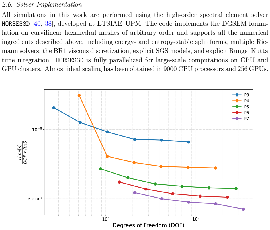
- [Abstract; §3.1; §5] The abstract claims the study is 'comparing lower- and very high-order configurations at similar degrees of freedom,' and §5 states that 'this issue is less pronounced at lower orders, where the inherent numerical damping partially compensates for the deficiencies of the model.' These cross-order claims are not supported by any experiment in the paper: all TGV simulations use a single 16^3 mesh and P=7 (§3.1), and the only P=3–7 data are the GPU throughput measurements in Fig. 1, which concern computational efficiency, not spectral fidelity or dissipation. The load-bearing condition for the abstract's practical guidance is that P=7 behavior is representative of very-high-order DG and that lower-order behavior at matched DOF follows the stated ordering. Since that condition is never tested, the generalization is an assertion. Either lower-order TGV runs at matched DOF must be added, or th
- [Abstract vs §6; §4.1.5] The abstract states, 'In the well-resolved cases considered, Vreman modeling does not improve accuracy because its active wavenumber range overlaps with the scheme's inherent dissipation.' This is internally inconsistent with the conclusions in §6, which recommend, for well-resolved LES in the turbulent regime, 'superior spectral fidelity is obtained using the split form and an LD-Roe flux, supplemented by an SGS model with a low constant (Cv = 0.01).' The same recommendation is supported by §4.1.5, where 'LD-Roe coupled with the Vreman model provides the best spectral fidelity.' These are not merely wording differences: one central message says Vreman is not helpful in well-resolved cases, while the other says the best well-resolved turbulent configuration uses Vreman. The abstract and conclusions need to be reconciled.
- [§4, Figs. 3–10] The accuracy assessments are made exclusively by visual inspection of dissipation-rate curves and energy spectra, without any quantitative error measure. This matters because the conclusions are finely graded: e.g., §4.1.3 claims that C_v=0.07 'over-dissipates energy at intermediate scales' while C_v=0.01 leaves the highest wavenumbers 'slightly under-dissipated'; §4.2.2 claims that C_v=0.01 'overestimates energy at intermediate wavenumbers.' Such claims are load-bearing for the proposed regime map and for the guidance in §6, but they rest on subjective comparison to reference spectra. The authors should provide quantitative metrics, for example relative L1/L2 errors of E(k) over defined wavenumber ranges or time-integrated dissipation-rate errors, so that 'best spectral fidelity' and 'over-dissipation' are defined operationally.
minor comments (5)
- [§4.1.2] The first sentence of §4.1.2 contains a typo: 'As in the reminder of the paper' should be 'As in the remainder of the paper.'
- [Fig. 3 caption] The caption says 'The standard and Morinishi schemes are shown only in Fig. 3a, as they became unstable before t/t_c = 9. Results for all schemes are shown in both figures' — this is self-contradictory. If standard and Morinishi are omitted from Fig. 3b, the sentence should say 'Results for all stable schemes are shown in both figures.'
- [§2.6; Fig. 1] The GPU efficiency metric Time/(DOF×RHS) is introduced without a definition of the RHS evaluation context (e.g., which flux/split form). Since the comparison spans P=3–7, a one-sentence statement of the test problem used for the benchmark would improve clarity.
- [§4.1.1] The standard versus split-form comparison uses Gauss nodes for the standard discretization and Gauss–Lobatto nodes for the split forms, so the effect of split-form stabilization is not isolated from the effect of nodal distribution. The text notes this, but a brief interpretive caution would be helpful for readers.
- [§6] The sentence 'Note that as only C_v = 0.01 and C_v = 0.07 were tested, the global optimum for this specific problem may lie within this range' is appropriate, but the bullet list should make explicit that the 'optimal' labels follow from only two constants, not from a true optimization over C_v.
Circularity Check
Numerical experiment with external references; not circular, though the broad regime claims are only weakly supported by a single P=7 case
-
renaming known result
[Sections 4.1.3 and 4.2.2 (Figures 9–10); conclusion in Section 6]
"increasing the constant to the typical finite-volume value of Cv = 0.07 aligns the spectrum around k = 20, but results in over-dissipation for k > 20."
The two-point sweep Cv ∈ {0.01, 0.07} is reframed as a finding about the 'optimal' constant lying in that range. This is a known-knob-tuning observation, not a derivation; it does not make the work circular because it is a posteriori description of an experiment, not a fitted input renamed as a prediction.
full rationale
The paper is a numerical experiment, not a derivation. Its target claims — that Vreman SGS is neutral in well-resolved high-order DG and helpful in under-resolved settings — are evaluated against external datasets (Bull & Jameson, Fehn et al., Carton de Wiart) rather than fitted from them. The Vreman constants are taken from the literature (Cv = 0.07 from finite-volume practice, Cv = 0.01 from high-order WRLES [31]) and only two values are swept; the paper explicitly states 'the global optimum for this specific problem may lie within this range,' so no fitted parameter is relabeled as a prediction. The abstract promises 'comparing lower- and very high-order configurations at similar degrees of freedom,' but the body only reports TGV simulations at P=7 on a fixed 16^3 mesh; the P=3–7 comparison exists only as a GPU-efficiency benchmark (Fig. 1), and the statement in Section 5 that 'this issue is less pronounced at lower orders' is asserted without supporting simulations. That is a representativeness/evidence gap, not a circularity: the conclusion is not entailed by its inputs by construction. Self-citations are present (e.g., HORSES3D [40, 38], Duan & Wang is external) but the central claim does not reduce to them. Score 1 reflects the minor, non-load-bearing gap between the abstract's lower-order framing and the actual P=7-only evidence, not a self-consistent derivation loop.
Assumptions & free parameters
free parameters (1)
- Vreman model constant C_v =
0.01 and 0.07 (tested, not fitted)
assumptions (5)
- standard math SBP-SAT split forms on Gauss-Lobatto nodes provide discrete energy/entropy stability and control aliasing.
- domain assumption The Vreman model with filter length Delta = V^(1/3)/(P+1) is an adequate representation of unresolved-scale dissipation in this DG formulation.
- domain assumption The external reference solutions (Bull & Jameson 512^3 DRP, Fehn et al. 8192^3, Carton de Wiart 512^3 pseudospectral) are accurate enough to judge spectral fidelity.
- domain assumption The Taylor-Green vortex at Re=1600 and in the inviscid limit is representative of well-resolved and under-resolved LES regimes relevant to GPU-oriented high-order DG.
- standard math The BR1 viscous discretization is neutrally stable and introduces minimal dissipation.
Cite this review
Pith. "Pith review of Can Explicit Subgrid Models Enhance Implicit LES Simulations? A Very High-Order Solver Perspective." pith.science (2026). https://pith.science/paper/I4LHGQSR
@misc{pith2026251204574,
  author       = {Pith},
  title        = {Pith review of: Can Explicit Subgrid Models Enhance Implicit LES Simulations? A Very High-Order Solver Perspective},
  year         = {2026},
  howpublished = {\url{https://pith.science/paper/I4LHGQSR}},
  note         = {Machine review of arXiv:2512.04574}
}
read the original abstract
High-order discontinuous Galerkin (DG) methods offer excellent accuracy for turbulent-flow simulations and are increasingly attractive on GPU-oriented architectures, where high polynomial orders can improve arithmetic intensity. However, very high-order under-resolved simulations remain sensitive to the balance between numerical and modeled dissipation. We investigate how explicit Vreman subgrid-scale (SGS) modeling interacts with dissipation from split-form stabilization and Riemann solvers in a DGSEM framework. Using the three-dimensional Taylor-Green vortex at Re=1600 and in the inviscid limit, we assess kinetic-energy dissipation, spectral accuracy, and stability across well-resolved, under-resolved viscous, and strongly under-resolved regimes, comparing lower- and very high-order configurations at similar degrees of freedom. The usefulness of explicit SGS modeling depends strongly on resolution, polynomial order, and the numerical dissipation already present. In the well-resolved cases considered, Vreman modeling does not improve accuracy because its active wavenumber range overlaps with the scheme's inherent dissipation. At similar degrees of freedom, lower-order simulations introduce stronger damping near the smallest resolved scales, whereas very high-order simulations preserve more spectral content but are more susceptible to high-wavenumber energy accumulation when dissipation is insufficient. Under stronger under-resolution, a weak SGS contribution can control this accumulation, while excessive SGS dissipation degrades intermediate scales. These results identify regimes in which explicit SGS modeling is beneficial, neutral, or detrimental, and provide practical guidance for selecting dissipation mechanisms in very high-order DG turbulence simulations suited to modern GPU architectures.
Figures


Figures from the paper (7 more)


Forward citations
Cited by 1 Pith paper
-
HORSES3D-GPU: A high-order discontinuous Galerkin solver for multi-GPU systems
HORSES3D was GPU-ported with OpenACC, achieving near-ideal scaling above ~16–20k elements per GPU and running a 2,048-GPU, 10.7B-DOF High-Lift Common Research Model simulation.
Reference graph
Works this paper leans on
-
[1]
J. S. Hesthaven, T. Warburton, Nodal Discontinuous Galerkin Methods, Springer NewYork, 2008.URL:https://doi.org/10.1007/978-0-387-72067-8.doi:10.1007/ 978-0-387-72067-8
-
[2]
Moura, S
R. Moura, S. Sherwin, J. Peiro, Eigensolution analysis of spectral/hp continuous Galerkin approximations to advection-diffusion problems: Insights into spectral van- ishing viscosity, Journal of Computational Physics 307 (2016) 401–422
2016
-
[3]
Sherwin, Dispersion analysis of the continuous and discontinuous Galerkin formula- tions., in: in International Symposium on Discontinuous Galerkin Methods, Springer, 1999, pp
S. Sherwin, Dispersion analysis of the continuous and discontinuous Galerkin formula- tions., in: in International Symposium on Discontinuous Galerkin Methods, Springer, 1999, pp. 425–431
1999
-
[4]
Manzanero, G
J. Manzanero, G. Rubio, E. Ferrer, E. Valero, Dispersion-dissipation analysis for ad- vection problems with nonconstant coefficients: Applications to discontinuous Galerkin formulations, SIAM Journal on Scientific Computing 40 (2018) A747–A768
2018
-
[5]
C. Canuto, M. Y. Hussaini, A. Quarteroni, T. A. Zang, Spectral Methods in Fluid Dynamics, Springer Berlin Heidelberg, 1988. URL:https://doi.org/10.1007/ 978-3-642-84108-8. doi:10.1007/978-3-642-84108-8
-
[6]
T. A. Zang, On the rotation and skew-symmetric forms for incompressible flow simula- tions, Applied Numerical Mathematics 7 (1991) 27–40
1991
-
[7]
Blaisdell, E
G. Blaisdell, E. Spyropoulos, J. Qin, The effect of the formulation of nonlinear terms on aliasing errors in spectral methods, Applied Numerical Mathematics 21 (1996) 207–219
1996
-
[8]
E. Ferrer, An interior penalty stabilised incompressible discontinuous Galerkin Fourier solver for implicit large eddy simulations, Journal of Computational Physics 348 (2017) 754 – 775. 24
2017
Show all 77 references
-
[9]
R. M. Kirby, S. J. Sherwin, Aliasing errors due to quadratic nonlinearities on triangular spectral /hp element discretisations, Journal of Engineering Mathematics 56 (2006) 273–288
2006
-
[10]
R. M. Kirby, G. E. Karniadakis, De-aliasing on non-uniform grids: algorithms and applications, Journal of Computational Physics 191 (2003) 249–264
2003
-
[11]
Mengaldo, D
G. Mengaldo, D. D. Grazia, D. Moxey, P. Vincent, S. Sherwin, Dealiasing techniques for high-order spectral element methods on regular and irregular grids, Journal of Computational Physics 299 (2015) 56–81
2015
-
[12]
H.Blackburn, S.Schmidt, Spectralelementfilteringtechniquesforlargeeddysimulation with dynamic estimation, Journal of Computational Physics 186 (2003) 610 – 629
2003
-
[13]
T. C. Fisher, M. H. Carpenter, High-order entropy stable finite difference schemes for nonlinear conservation laws: Finite domains, Journal of Computational Physics 252 (2013) 518–557
2013
-
[14]
M. H. Carpenter, T. C. Fisher, E. J. Nielsen, S. H. Frankel, Entropy stable spectral collocation schemes for the Navier–Stokes equations: Discontinuous interfaces, SIAM Journal on Scientific Computing 36 (2014) B835–B867
2014
-
[15]
Schwarz, D
A. Schwarz, D. Kempf, J. Keim, P. Kopper, C. Rohde, A. Beck, Comparison of entropy stable collocation high-order DG methods for compressible turbulent flows, Computers & Fluids 303 (2025) 106874
2025
-
[16]
Manzanero, G
J. Manzanero, G. Rubio, D. A. Kopriva, E. Ferrer, E. Valero, An entropy–stable discon- tinuous Galerkin approximation for the incompressible Navier–Stokes equations with variable density and artificial compressibility, Journal of Computational Physics 408 (2020) 109241
2020
-
[17]
Manzanero, G
J. Manzanero, G. Rubio, D. A. Kopriva, E. Ferrer, E. Valero, A free–energy stable nodal discontinuous Galerkin approximation with summation–by–parts property for the Cahn–Hilliard equation, Journal of Computational Physics 403 (2020) 109072
2020
-
[18]
Lodares, J
D. Lodares, J. Manzanero, E. Ferrer, E. Valero, An entropy–stable discontinuous Galerkin approximation of the Spalart–Allmaras turbulence model for the compress- ible Reynolds Averaged Navier–Stokes equations, Journal of Computational Physics 455 (2022) 110998. 25
2022
-
[19]
Ntoukas, J
G. Ntoukas, J. Manzanero, G. Rubio, E. Valero, E. Ferrer, A free–energy stable p– adaptive nodal discontinuous Galerkin for the Cahn–Hilliard equation, Journal of Com- putational Physics 442 (2021) 110409
2021
-
[20]
G.Ntoukas, J.Manzanero, G.Rubio, E.Valero, E.Ferrer, Anentropy–stablep–adaptive nodal discontinuous Galerkin for the coupled Navier–Stokes/Cahn–Hilliard system, Journal of Computational Physics 458 (2022) 111093
2022
-
[21]
A. R. Winters, R. C. Moura, G. Mengaldo, G. J. Gassner, S. Walch, J. Peiro, S. J. Sherwin, A comparative study on polynomial dealiasing and split form discontinuous Galerkin schemes for under-resolved turbulence computations, Journal of Computa- tional Physics 372 (2018) 1–21
2018
-
[22]
Smagorinsky, General circulation experiments with the primitive equations: I
J. Smagorinsky, General circulation experiments with the primitive equations: I. the basic experiment, Monthly weather review 91 (1963) 99–164
1963
-
[23]
D. K. Lilly, On the computational stability of numerical solutions of time-dependent non-linear geophysical fluid dynamics problems, Monthly Weather Review 93 (1965) 11–25
1965
-
[24]
Nicoud, F
F. Nicoud, F. Ducros, Subgrid-scale stress modelling based on the square of the velocity gradient tensor, Flow, turbulence and Combustion 62 (1999) 183–200
1999
-
[25]
Vreman, An eddy-viscosity subgrid-scale model for turbulent shear flow: Algebraic theory and applications, Physics of fluids 16 (2004) 3670–3681
A. Vreman, An eddy-viscosity subgrid-scale model for turbulent shear flow: Algebraic theory and applications, Physics of fluids 16 (2004) 3670–3681
2004
-
[26]
D. J. Garmann, M. R. Visbal, P. D. Orkwis, Comparative study of implicit and subgrid- scale model large-eddy simulation techniques for low-Reynolds number airfoil applica- tions, International Journal for Numerical Methods in Fluids 71 (2013) 1546–1565
2013
-
[27]
Y. Li, Z. Wang, A priori and a posteriori evaluations of sub-grid scale models for the Burgers’ equation, Computers & Fluids 139 (2016) 92–104
2016
-
[28]
Z. Duan, Z. Wang, Calibrating sub-grid scale models for high-order wall-modeled large eddy simulation, Advances in Aerodynamics 6 (2024) 5
2024
-
[29]
Chatterjee, Y
T. Chatterjee, Y. T. Peet, Effect of artificial length scales in large eddy simulation of a neutral atmospheric boundary layer flow: A simple solution to log-layer mismatch, Physics of Fluids 29 (2017) 075105. 26
2017
-
[30]
Mukha, P
T. Mukha, P. Schlatter, Wall-modeled large-eddy simulation based on spectral-element discretization, arXiv preprint arXiv:2404.05378 (2024)
2024 arXiv
-
[31]
Kumar, O
V. Kumar, O. Lehmkuhl, A. Tomboulides, P. Fischer, M. Min, Turbulence Modeling with Nek5000/RS, SOD2D and Alya, Technical Report, Argonne National Laboratory (ANL), Argonne, IL (United States), 2023
2023
-
[32]
Reddy, Y
S. Reddy, Y. Tissaoui, Comparison of sub-grid scale models for large-eddy simulation using a high-order spectral element approximation of the compressible Navier-Stokes equations at low Mach number, Technical Report, 2021
2021
-
[33]
Ntoukas, G
G. Ntoukas, G. Rubio, O. A. Marino, A. Liosi, F. Bottone, J. Hoessler, E. Ferrer, A comparative study of explicit and implicit large eddy simulations using a high-order discontinuous Galerkin solver: Application to a Formula 1 front wing, Results in Engi- neering 25 (2025) 104425
2025
-
[34]
A. Beck, M. Kurz, Toward discretization-consistent closure schemes for large eddy simulation using reinforcement learning, Physics of Fluids 35 (2023) 125122
2023
-
[35]
M. Kurz, P. Offenhäuser, A. Beck, Deep reinforcement learning for turbulence modeling in large eddy simulations, International Journal of Heat and Fluid Flow 99 (2023) 109094
2023
-
[36]
N. Fehn, W. A. Wall, M. Kronbichler, Efficiency of high-performance discontinuous Galerkin spectral element methods for under-resolved turbulent incompressible flows, International Journal for Numerical Methods in Fluids 88 (2018) 32–54
2018
-
[37]
Gasparino, F
L. Gasparino, F. Spiga, O. Lehmkuhl, SOD2D: A GPU-enabled spectral finite elements method for compressible scale-resolving simulations, Computer Physics Communica- tions 297 (2024) 109067
2024
-
[38]
Accessed: 2025-09-30
HORSES3D: A high-order discontinuous Galerkin solver for flow simulations and multi- physics applications,https://github.com/loganoz/horses3d-gpu, 2025. Accessed: 2025-09-30
2025
-
[39]
Kopriva, Implementingspectralmethodsforpartialdifferentialequations, Springer Netherlands, 2009
D.A. Kopriva, Implementingspectralmethodsforpartialdifferentialequations, Springer Netherlands, 2009. URL:http://dx.doi.org/10.1007/978-90-481-2261-5. doi:10. 1007/978-90-481-2261-5. 27
2009 doi
-
[40]
Ferrer, G
E. Ferrer, G. Rubio, G. Ntoukas, W. Laskowski, O. A. Mariño, S. Colombo, A. Mateo- Gabín, H. Marbona, F. M. de Lara, D. Huergo, et al., HORSES3D: A high-order discon- tinuous Galerkin solver for flow simulations and multi-physics applications, Computer Physics Communications 2...
2023
-
[41]
Gassner, D
G. Gassner, D. A. Kopriva, A comparison of the dispersion and dissipation errors of Gauss and Gauss–Lobatto discontinuous Galerkin spectral element methods, SIAM Journal on Scientific Computing 33 (2011) 2560–2579
2011
-
[42]
Manzanero, A
J. Manzanero, A. M. Rueda-Ramírez, G. Rubio, E. Ferrer, The Bassi Rebay 1 scheme is a special case of the symmetric interior penalty formulation for discontinuous Galerkin discretisationswithGauss–Lobattopoints, JournalofComputationalPhysics363(2018) 1–10
2018
-
[44]
Arnold, F
D. Arnold, F. Brezzi, B. Cockburn, L. Marini, Unified analysis of discontinuous Galerkin methods for elliptic problems, SIAM Journal of Numerical Analysis 39 (2001) 1749– 1779
2001
-
[45]
G. J. Gassner, A. D. Beck, On the accuracy of high-order discretizations for under- resolved turbulence simulations, Theoretical and Computational Fluid Dynamics 27 (2012) 221–237
2012
-
[46]
Kopriva and G.J
D.A. Kopriva and G.J. Gassner, An energy stable discontinuous Galerkin spectral element discretization for variable coefficient advection problems, SIAM Journal on Scientific Computing 36 (2014) A2076–A2099
2014
-
[47]
G. J. Gassner, A. R. Winters, D. A. Kopriva, Split form nodal discontinuous Galerkin schemes with summation-by-parts property for the compressible Euler equations, Jour- nal of Computational Physics 327 (2016) 39–66
2016
-
[48]
Manzanero, G
J. Manzanero, G. Rubio, E. Ferrer, E. Valero, D. A. Kopriva, Insights on aliasing driven instabilities for advection equations with application to Gauss-Lobatto discontinuous Galerkin methods, J. Sci. Comput. 75 (2018) 1262–1281
2018
-
[49]
Mateo-Gabín, A
A. Mateo-Gabín, A. M. Rueda-Ramírez, E. Valero, G. Rubio, A flux-differencing for- mulation with Gauss nodes, Journal of Computational Physics 489 (2023) 112298. 28
2023
-
[50]
D. A. Kopriva, G. J. Gassner, An energy stable discontinuous Galerkin spectral element discretization for variable coefficient advection problems, SIAM Journal on Scientific Computing 36 (2014) A2076–A2099
2014
-
[51]
G. J. Gassner, A. R. Winters, F. J. Hindenlang, D. A. Kopriva, The BR1 scheme is stable for the compressible Navier–Stokes equations, Journal of Scientific Computing 77 (2018) 154–200
2018
-
[52]
Manzanero, G
J. Manzanero, G. Rubio, D. A. Kopriva, E. Ferrer, E. Valero, Entropy–stable discontin- uous Galerkin approximation with summation–by–parts property for the incompressible Navier–Stokes/Cahn–Hilliard system, Journal of Computational Physics (2020) 109363
2020
-
[53]
Chen, C.-W
T. Chen, C.-W. Shu, Entropy stable high order discontinuous Galerkin methods with suitable quadrature rules for hyperbolic conservation laws, Journal of Computational Physics 345 (2017) 427–461
2017
-
[54]
G. J. Gassner, A skew-symmetric discontinuous Galerkin spectral element discretization and its relation to SBP-SAT finite difference methods, SIAM Journal on Scientific Computing 35 (2013) A1233–A1253
2013
-
[55]
A. R. Winters, D. A. Kopriva, G. J. Gassner, F. Hindenlang, Construction of modern robust nodal discontinuous Galerkin spectral element methods for the compressible Navier–Stokes equations, in: Efficient High-Order Discretizations for Computational Fluid Dynamics, Springer, 20...
2021
-
[56]
Chen, C.-W
T. Chen, C.-W. Shu, Review of entropy stable discontinuous Galerkin methods for systems of conservation laws on unstructured simplex meshes, CSIAM Trans. Appl. Math. 1 (2020) 1–52
2020
-
[57]
Y. Morinishi, Skew-symmetric form of convective terms and fully conservative finite dif- ference schemes for variable density low-mach number flows, Journal of Computational Physics 229 (2010) 276–300
2010
-
[58]
Ducros, F
F. Ducros, F. Laporte, T. Soulères, V. Guinot, P. Moinat, B. Caruelle, High-order fluxes for conservative skew-symmetric-like schemes in structured meshes: Application to compressible flows, Journal of Computational Physics 161 (2000) 114–139
2000
-
[59]
C. A. Kennedy, A. Gruber, Reduced aliasing formulations of the convective terms within the Navier–Stokes equations for a compressible fluid, Journal of Computational Physics 227 (2008) 1676–1700. 29
2008
-
[60]
Pirozzoli, Generalized conservative approximations of split convective derivative operators, Journal of Computational Physics 229 (2010) 7180–7190
S. Pirozzoli, Generalized conservative approximations of split convective derivative operators, Journal of Computational Physics 229 (2010) 7180–7190
2010
-
[61]
Ismail, P
F. Ismail, P. L. Roe, Affordable, entropy-consistent euler flux functions II: Entropy production at shocks, Journal of Computational Physics 228 (2009) 5410–5436
2009
-
[62]
P. Chandrashekar, Kinetic energy preserving and entropy stable finite volume schemes for compressible Euler and Navier-Stokes equations, Communications in Computational Physics 14 (2013) 1252–1286
2013
-
[63]
Z. Wang, R. Fidkowski, K.and Abgrall, F. Bassi, D. Caraeni, A. Cary, H. Deconinck, R. Hartmann, K. Hillewaert, H. Huynh, N. Kroll, G. May, P. Persson, B. van Leer, M. Visbal, High-order CFD methods: current status and perspective, International Journal for Numerical Methods in...
2013
-
[64]
A. Beck, T. Bolemann, D. Flad, H. Frank, G. Gassner, F. Hindenlang, C. Munz, High- order discontinuous Galerkin spectral element methods for transitional and turbulent flow simulations, International Journal for Numerical Methods in Fluids 76 (2014) 522–548
2014
-
[65]
D. Flad, G. Gassner, On the use of kinetic energy preserving DG-schemes for large eddy simulation, Journal of Computational Physics 350 (2017) 782 – 795
2017
-
[66]
Manzanero, E
J. Manzanero, E. Ferrer, G. Rubio, E. Valero, On the role of numerical dissipation in stabilising under-resolved turbulent simulations using discontinuous Galerkin methods, arXiv:1805.10519 (2018)
2018 arXiv
-
[67]
E. F. Toro, Riemann solvers and numerical methods for fluid dynamics: a practical introduction, Springer Science & Business Media, 2013
2013
-
[68]
Oßwald, A
K. Oßwald, A. Siegmund, P. Birken, V. Hannemann, A. Meister, L2Roe: a low dissipa- tion version of roe’s approximate riemann solver for low mach numbers, International Journal for Numerical Methods in Fluids 81 (2016) 71–86
2016
-
[69]
K. O. Friedrichs, P. D. Lax, Systems of conservation equations with a convex extension, Proceedings of the National Academy of Sciences 68 (1971) 1686–1688
1971
-
[70]
Williamson, Low-storage Runge-Kutta schemes, Journal of Computational Physics 35 (1980) 48–56
J. Williamson, Low-storage Runge-Kutta schemes, Journal of Computational Physics 35 (1980) 48–56. 30
1980
-
[71]
N. Fehn, M. Kronbichler, P. Munch, W. A. Wall, Numerical evidence of anomalous energy dissipation in incompressible Euler flows: towards grid-converged results for the inviscid taylor–green problem, Journal of Fluid Mechanics 932 (2022) A40
2022
-
[72]
J. R. Bull, A. Jameson, Simulation of the Taylor–Green vortex using high-order flux reconstruction schemes, AIAA Journal 53 (2015) 2750–2761
2015
-
[73]
Carton De Wiart, K
C. Carton De Wiart, K. Hillewaert, M. Duponcheel, G. Winckelmans, Assessment of a discontinuous Galerkin method for the simulation of vortical flows at high Reynolds number, International Journal for Numerical Methods in Fluids 74 (2014) 469–493
2014
-
[74]
Mateo-Gabin, K
A. Mateo-Gabin, K. Tlales, E. Valero, E. Ferrer, G. Rubio, An unsupervised machine- learning-based shock sensor: Application to high-order supersonic flow solvers, Expert Systems with Applications 270 (2025) 126352
2025
-
[75]
Vázquez, G
M. Vázquez, G. Houzeaux, S. Koric, A. Artigues, J. Aguado-Sierra, R. Arís, D. Mira, H. Calmet, F. Cucchietti, H. Owen, et al., Alya: Multiphysics engineering simulation toward exascale, Journal of computational science 14 (2016) 15–27
2016
-
[76]
Manzanero, E
J. Manzanero, E. Ferrer, G. Rubio, E. Valero, Design of a Smagorinsky spectral van- ishing viscosity turbulence model for discontinuous Galerkin methods, Computers & Fluids 200 (2020) 104440
2020
-
[77]
R. C. Moura, G. Mengaldo, J. Peiró, S. J. Sherwin, An LES setting for DG-based implicit LES with insights on dissipation and robustness, in: Spectral and High Order Methods for Partial Differential Equations ICOSAHOM 2016, Springer, 2017, pp. 161– 173
2016
-
[78]
R. M. Kirby, S. J. Sherwin, Stabilisation of spectral/hp element methods through spec- tral vanishing viscosity: Application to fluid mechanics modelling, Computer methods in applied mechanics and engineering 195 (2006) 3128–3144. 31
2006
Reviewed August 3, 2026 · model on record in the stance chip above.
Discussion (0). Continue with ORCID to comment.