REVIEW 3 major objections 4 minor 12 references
Statistical Physics of Deep Neural Networks: Generalization Capability, Beyond the Infinite Width, and Feature Learning
T0 review · 3 major / 4 minor · reviewed 2026-08-09 · deepseek-v4-flash
Pith's one-line read A statistical-mechanics bound says deep networks generalize by last-layer width alone.
desk verdict Real result for random-feature readouts, dressed up as a general deep-learning bound; the scope gap is the decisive weakness. read the letter →
The pith
A machine-rendered reading of the paper's core claim, the machinery that carries it, and where it could break.
The reading
What carries the argument
The central machinery is the quenched average of the partition function for a network split into a fixed random feature map and a trained last layer, evaluated with the replica trick under a replica-symmetric ansatz. A Gaussian approximation of the residuals between predictions and labels turns the disorder average into a tractable integral whose saddle-point equations yield order parameters from which both generalization and training errors are read off.
What would settle it
One could settle the central claim by training a family of deep networks with identical last-layer width and widely varying hidden-layer widths on the same regression task: if the generalization gap grows with hidden-layer width in the large-sample limit, the last-layer-only bound is wrong. A complementary check is to measure the non-Gaussianity of the training residuals, since the derivation's Gaussian step predicts those higher cumulants should vanish.
Extended reading notes
Core claim
The paper's central claim is that when the hidden layers of a deep network are treated as fixed random features and only the last layer is optimized, the average generalization gap is set by the number of output-layer neurons—not by the total number of trainable weights. Using the replica method, the thesis derives closed expressions for generalization and training errors, and shows that in the large-data, large-width limit the bound improves on worst-case capacity bounds by orders of magnitude. The same data-dependent framework yields a finite-width thermodynamic limit with a closed-form generalization error for a one-hidden-layer network, and identifies deep networks in this regime with Student's t-processes. The final part examines a controlled teacher-student task and finds conditions under which networks collapse to the teacher—learning structure—rather than memorizing the dataset.
Load-bearing premise
The bound assumes that hidden layers act as fixed random feature generators and that the deviations between predictions and labels can be treated as Gaussian, an approximation the paper itself calls 'somewhat uncontrolled'.
Editorial extensions
If this is right
- In the asymptotic regime, the generalization gap of a deep network with an optimized readout is controlled by the last layer width and the number of samples, not the full parameter count.
- The bound improves on worst-case capacity bounds by several orders of magnitude for typical large networks.
- A closed-form generalization error exists for finite-width one-hidden-layer networks in the proportional regime where sample count scales with width.
- Deep networks in this thermodynamic limit are statistically equivalent to Student's t-processes, giving a tractable non-Gaussian prior beyond the infinite-width Gaussian process.
- Under a controlled teacher-student task, the volume of solutions and Gaussianity breaking determine whether a network learns the teacher's structure or merely memorizes training labels.
Reading between the lines
- One consequence not spelled out in the thesis is a 'readout bottleneck' principle: if the last-layer-only bound survives fully trained hidden layers, then deep representations store information that a small readout can exploit, so generalization capacity is set by the readout rather than by the whole network.
- The link to Student's t-processes suggests a testable prediction for Bayesian deep learning: finite-width posteriors should show heavier tails than their infinite-width Gaussian-process limits, with the tails controlled by network width and depth.
- The Gaussian approximation flagged as uncontrolled in the thesis could be tested directly by computing the fourth cumulant of residual distributions in numerical experiments; a large deviation from zero in the proportional regime would signal where the bound should break down.
- The memorize-vs-learn criterion from the final chapter could be turned into a practical probe: measure solution-space volume or Gaussianity breaking on real datasets to detect when a model is forced to internalize data structure.
Editorial analysis
A structured set of objections, weighed in public.
Referee Report
Summary. The thesis applies equilibrium statistical-mechanics methods to deep neural networks. Chapter 2 develops a teacher-student regression model in which the first L-1 layers are treated as a frozen random feature map and only the last-layer weights are optimized; a replica calculation yields average training and generalization errors (Eqs. 2.52, 2.54) and an asymptotic bound that the abstract advertises as depending only on the last-layer width. Chapter 3 studies a finite-width, proportional thermodynamic limit beyond the infinite-width regime and reports a closed-form generalization error for one-hidden-layer networks, an approximate partition function for deeper networks, and a connection to Student-t processes. Chapter 4 presents a preliminary task-explicit analysis of when a network learns an internal representation of the teacher rather than memorizing the training set.
Significance. Chapter 2's saddle-point formulas are genuinely parameter-free: no constants are fitted, and the numerical tests in Section 2.3.1 provide evidence that the bound tracks simulated generalization gaps. Chapter 3's closed-form finite-width generalization error is a constructive step beyond the infinite-width limit. If the advertised last-layer-only bound applied to fully trained deep networks, it would be a major improvement over VC/Rademacher bounds. However, the derivation in Chapter 2 is for a random-feature model with readout-only training, and the extension to fully trained networks is asserted rather than proved; this scope gap is the main weakness. The thesis is therefore best read as a technically rich contribution to random-feature and finite-width statistical mechanics, with the fully trained DNN claim currently an overreach.
major comments (3)
- [§2.2.1, Eq. (2.18); Abstract and §0.2] The central derivation starts from f_DNN(x)=v·φ(x) with only v optimized and φ a fixed (random) feature map, and the text explicitly says 'we assume fixed (and random) features and only optimize the last layer weights.' The abstract and introduction, however, state the result for deep networks in general: the generalization bound 'only depends on the last layer size rather than on the total number of network parameters.' No theorem, coupling bound, or monotonicity argument is provided showing that end-to-end training of hidden layers preserves or improves the frozen-feature bound. The order parameters J and Φ in Eq. (2.26) are functionals of the feature map; training the hidden layers changes them, and the generalization gap is not monotone under enlarging the hypothesis class. The statement in §2.1.4 that the formulas apply to a subspace 'which, we will argue, contains trained networks' is not backed by an argument in the visible text. As written, the result is a statement about random-feature/readout-only models; either add a quantitative transfer argument (e.g., a lazy-training/NTK regime) or explicitly restrict the claim and adjust the abstract accordingly.
- [§2.2.2, Eqs. (2.24)–(2.27), (2.40)] The Gaussian approximation for the joint distribution of residuals q_a is load-bearing: it is used to evaluate the dataset integral in Eq. (2.27) and enters the action in Eq. (2.40), from which Eqs. (2.52) and (2.54) follow. The text itself calls this approximation 'somewhat uncontrolled' and justifies it only by analogy with the Gaussian equivalence principle and weak mutual correlations of the feature map. The manuscript should state the precise scaling/normalization conditions under which the approximation is controlled, or quantify its failure through finite-N corrections or additional numerical checks. Without this, the asymptotic bound is a plausible mean-field result rather than a proved statement.
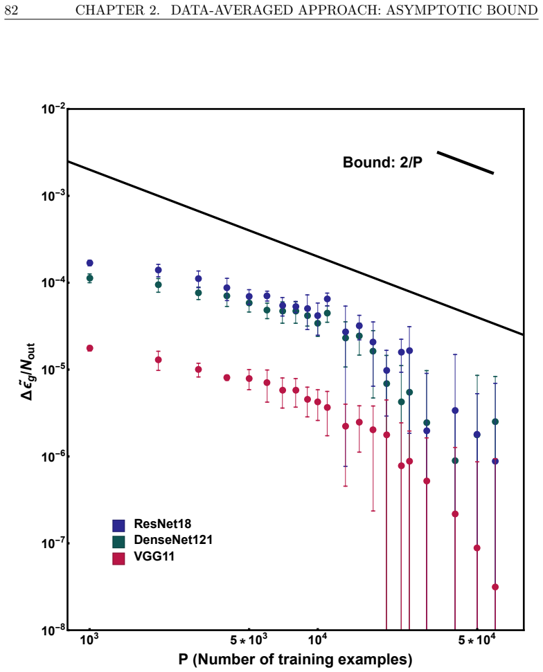
- [§2.3.1] The numerical tests appear to include state-of-the-art architectures trained end-to-end on real datasets, while the theoretical formulas were derived for readout-only training on frozen features. Empirical agreement for fully trained networks is encouraging but does not substitute for a derivation; the manuscript should separate 'derived for frozen features' from 'observed for fully trained networks,' and should discuss why the bound may survive feature learning (e.g., because deep features approach a random-feature or lazy-training regime in the tested settings).
minor comments (4)
- [§2.1.3, Theorem 2.1.2] The Rademacher bound contains a minus sign before the square-root term; a negative term would make the upper bound potentially negative, so the sign should be checked (the standard form has a positive confidence term).
- [§2.2.2, gray-box details] The notation in the Gaussian and Hubbard-Stratonovich integrals is inconsistent, with missing normalization factors in some of the z-integrals; please clean up this derivation for readability.
- [§2.4 heading] The section title 'Discussion and prespective' contains a typo; it should read 'Discussion and perspective.'
- [Abstract and Eq. (2.52)] The phrase 'only depends on the last layer size' should be reconciled with Eq. (2.52), where J and Φ depend on the feature map; please specify precisely whether the dependence on hidden-layer widths and weight distributions is absent asymptotically or merely not tracked.
Circularity Check
No direct circular reduction; the last-layer bound is a genuine consequence of the explicit readout-only model, but the paper's headline claim about fully trained DNNs is a scope extrapolation, and the one self-citation is not load-bearing.
full rationale
The central derivation in Chapter 2 is self-contained for the model as defined: Eqs. (2.18), (2.22), (2.49), (2.52), and (2.54) follow from a quenched replica saddle-point calculation for a teacher-student problem with fixed random features and only the last-layer weights optimized. No fitted constants are introduced, and the generalization and training errors are not defined to equal the claimed bound. The dependence on the last-layer size N is a consequence of the model, since only the readout v of size N is trainable, so the statement that the bound depends on last-layer size rather than total parameter count is an artifact of that readout-only assumption rather than an independent discovery about fully trained DNNs. This is a scope limitation, not a circularity: the random-feature result is honestly derived for the stated model, while the transfer to fully trained networks is asserted without a theorem. The Gaussian approximation is explicitly flagged as 'somewhat uncontrolled due to the absence of a formal result confirming its validity' and is justified by external prior work (e.g., the Gaussian equivalence principle), not by a self-citation chain. The only identifiable self-citation, '[APG+22]' in the Chapter 2 introduction ('as further discussed in [APG+22]'), is a pointer to related discussion and is not load-bearing for any equation. No self-definitional equality, fitted parameter renamed as prediction, or imported uniqueness theorem was found.
Assumptions & free parameters
assumptions (4)
- domain assumption Inputs are iid draws from rho(x) and labels come from a teacher f_T(x).
- domain assumption The joint distribution of q_a = f_T - v dot phi can be approximated as multivariate Gaussian, the Gaussian equivalence principle.
- domain assumption The replica trick with a replica symmetric ansatz is valid, with convexity of the last-layer problem making the ansatz exact.
- ad hoc to paper Only the last layer is trained; hidden features are fixed random maps, and trained DNNs are argued to lie in this subspace.
Cite this review
Pith. "Pith review of Statistical Physics of Deep Neural Networks: Generalization Capability, Beyond the Infinite Width, and Feature Learning." pith.science (2026). https://pith.science/paper/L6SVVYMG
@misc{pith2026250119281,
  author       = {Pith},
  title        = {Pith review of: Statistical Physics of Deep Neural Networks: Generalization Capability, Beyond the Infinite Width, and Feature Learning},
  year         = {2026},
  howpublished = {\url{https://pith.science/paper/L6SVVYMG}},
  note         = {Machine review of arXiv:2501.19281}
}
read the original abstract
Deep Neural Networks (DNNs) excel at many tasks, often rivaling or surpassing human performance. Yet their internal processes remain elusive, frequently described as "black boxes." While performance can be refined experimentally, achieving a fundamental grasp of their inner workings is still a challenge. Statistical Mechanics has long tackled computational problems, and this thesis applies physics-based insights to understand DNNs via three complementary approaches. First, by averaging over data, we derive an asymptotic bound on generalization that depends solely on the size of the last layer, rather than on the total number of parameters -- revealing how deep architectures process information differently across layers. Second, adopting a data-dependent viewpoint, we explore a finite-width thermodynamic limit beyond the infinite-width regime. This leads to: (i) a closed-form expression for the generalization error in a finite-width one-hidden-layer network (regression task); (ii) an approximate partition function for deeper architectures; and (iii) a link between deep networks in this thermodynamic limit and Student's t-processes. Finally, from a task-explicit perspective, we present a preliminary analysis of how DNNs interact with a controlled dataset, investigating whether they truly internalize its structure -- collapsing to the teacher -- or merely memorize it. By understanding when a network must learn data structure rather than just memorize, it sheds light on fostering meaningful internal representations. In essence, this thesis leverages the synergy between Statistical Physics and Machine Learning to illuminate the inner behavior of DNNs.
Figures


Figures from the paper (29 more)




Reference graph
Works this paper leans on
-
[6]
doi: 10 . 1088 / 1751 - 8121 / aba028. url: https : / / doi . org / 10 . 1088/1751-8121/aba028. [CUH16] Djork-Arne Clevert, Thomas Unterthiner, and Sepp Hochreiter. Fast and accurate deep network learning by exponential linear units (elus).arXiv preprint arXiv:1511.07289, 2016. [CV95] Corinna Cortes and Vladimir Vapnik. Support-vector networks. Machine Le...
arXiv 2016
-
[296]
[YSL+13] Dong Yu, Michael L Seltzer, Jinyu Li, Jui-Ting Huang, and Frank Seide
IEEE, 2015. [YSL+13] Dong Yu, Michael L Seltzer, Jinyu Li, Jui-Ting Huang, and Frank Seide. Feature learning in deep neural networks-studies on speech recognition tasks. arXiv preprint arXiv:1301.3605, 2013. [YYY+20] Zitong Yang, Yaodong Yu, Chong You, Jacob Steinhardt, and Yi Ma. Re- thinking bias-variance trade-off for generalization of neural networks....
arXiv 2015
-
[362]
[RHW86b] David E Rumelhart, Geoffrey E Hinton, and Ronald J Williams
MIT Press, 1986. [RHW86b] David E Rumelhart, Geoffrey E Hinton, and Ronald J Williams. Learn- ing representations by back-propagating errors.nature, 323(6088):533–536, 1986. [RIG23] Maria Refinetti, Alessandro Ingrosso, and Sebastian Goldt. Neural net- works trained with SGD learn distributions of increasing complexity. In Andreas Krause, Emma Brunskill, ...
arXiv 1986
-
[1530]
[AGS87] Daniel J Amit, Hanoch Gutfreund, and Haim Sompolinsky
url: https://link.aps.org/doi/10.1103/PhysRevLett.55.1530. [AGS87] Daniel J Amit, Hanoch Gutfreund, and Haim Sompolinsky. Statistical me- chanics of neural networks near saturation.Annals of physics, 173(1):30– 67, 1987. [Ait20] Laurence Aitchison. Why bigger is not always better: on finite and infinite neural networks. In Hal Daumé III and Aarti Singh, e...
-
[1983]
url: https ://www.sciencedirect.com/science/article/pii/0047259X83900192
issn: 0047-259X.doi: 10.1016/0047-259X(83)90019-2. url: https ://www.sciencedirect.com/science/article/pii/0047259X83900192. [BMZ19] Carlo Baldassi, Enrico M. Malatesta, and Riccardo Zecchina. Properties of the geometry of solutions and capacity of multilayer neural networks with rectified linear unit activations.Phys. Rev. Lett., 123:170602, 17, October
-
[1999]
187 [GSJ+20] Mario Geiger, Stefano Spigler, Arthur Jacot, and Matthieu Wyart
doi: 10.1162/089976699300016629. 187 [GSJ+20] Mario Geiger, Stefano Spigler, Arthur Jacot, and Matthieu Wyart. Dis- entangling feature and lazy training in deep neural networks.Journal of Statistical Mechanics: Theory and Experiment, 2020(11):113301, 2020. [GSS14] Ian J Goodfellow, Jonathon Shlens, and Christian Szegedy. Explaining and harnessing adversar...
-
[2014]
[SZ14] Karen Simonyan and Andrew Zisserman
url: https://proceedings.mlr.press/v33/shah14.html. [SZ14] Karen Simonyan and Andrew Zisserman. Very deep convolutional networks for large-scale image recognition.arXiv preprint arXiv:1409.1556, 2014. [TDC86] Gerard Toulouse, Stanislas Dehaene, and Jean-Pierre Changeux. Spin glass model of learning by selection. Proceedings of the National Academy of Scie...
arXiv 2014
-
[2017]
[LBB+98] Yann LeCun, Leon Bottou, Yoshua Bengio, and Patrick Haffner
doi: 10.1038/s41467-017-01596-3. [LBB+98] Yann LeCun, Leon Bottou, Yoshua Bengio, and Patrick Haffner. Gradient- based learning applied to document recognition.Proceedings of the IEEE, 86(11):2278–2324, 1998. doi: 10.1109/5.726791. [LBN+17a] Jaehoon Lee, Yasaman Bahri, Roman Novak, Samuel S Schoenholz, Jeffrey Pennington, and Jascha Sohl-Dickstein. Deep n...
arXiv 1998
Show all 12 references
-
[2018]
url: https://link.aps.org/ doi/10.1103/PhysRevX.8.031003
doi: 10.1103/PhysRevX.8.031003. url: https://link.aps.org/ doi/10.1103/PhysRevX.8.031003. [COB19a] Lenaic Chizat, Edouard Oyallon, and Francis Bach. On lazy training in differentiable programming. In H. Wallach, H. Larochelle, A. Beygelzimer, F. d’Alche-Buc, E. Fox, and R. Gar...
-
[2019]
url: https://link.aps
doi: 10.1103/PhysRevLett.123.170602. url: https://link.aps. org/doi/10.1103/PhysRevLett.123.170602. [Bot10] Léon Bottou. Large-scale machine learning with stochastic gradient de- scent. InProceedings of COMPSTAT’2010, pages 177–186. Springer, 2010. 182 CHAPTER 6. BIBLIOGRAPHY ...
2010 arXiv
-
[2020]
url: https://proceedings.mlr.press/v119/aitchison20a.html. [AJB+17] Devansh Arpit, Stanislaw Jastrzebski, Nicolas Ballas, David Krueger, Em- manuel Bengio, Maxinder S Kanwal, Tegan Maharaj, Asja Fischer, Aaron Courville, Yoshua Bengio, et al. A closer look at memorization in d...
2017 arXiv
-
[2021]
url: https://link.aps
doi: 10.1103/PhysRevE.103.042142 . url: https://link.aps. org/doi/10.1103/PhysRevE.103.042142. 192 CHAPTER 6. BIBLIOGRAPHY [Mur12] Kevin P. Murphy. Machine Learning: A Probabilistic Perspective. MIT Press, 2012. [MV15] Aravindh Mahendran and Andrea Vedaldi. Understanding deep ...
2012
Reviewed August 9, 2026 · model on record in the stance chip above.
Discussion (0). Continue with ORCID to comment.