Detecting entanglement of non-Gaussian continuous-variable states from single-copy homodyne measurements
Pith reviewed 2026-06-30 10:10 UTC · model grok-4.3
The pith
Randomized homodyne data on single copies yields estimators for partial-transpose moments that detect non-Gaussian CV entanglement.
A machine-rendered reading of the paper's core claim, the machinery that carries it, and where it could break.
Core claim
Unbiased U-statistic estimators for the partial-transpose moments p2 and p3 can be constructed from randomized homodyne quadrature data on a single copy; these estimators evaluate the p3-PPT entanglement witnesses and thereby detect bipartite CV entanglement while also furnishing a dimension-free lower bound on negativity, with sample complexity O((N+1)^{14/3}/ε²) for additive error ε at Fock cutoff N.
What carries the argument
Unbiased U-statistic estimators for the partial-transpose moments p2 and p3 constructed from randomized single-copy homodyne quadrature data.
If this is right
- Both a linear witness for detection and a quadratic witness yielding a dimension-free negativity lower bound become evaluable from the same data.
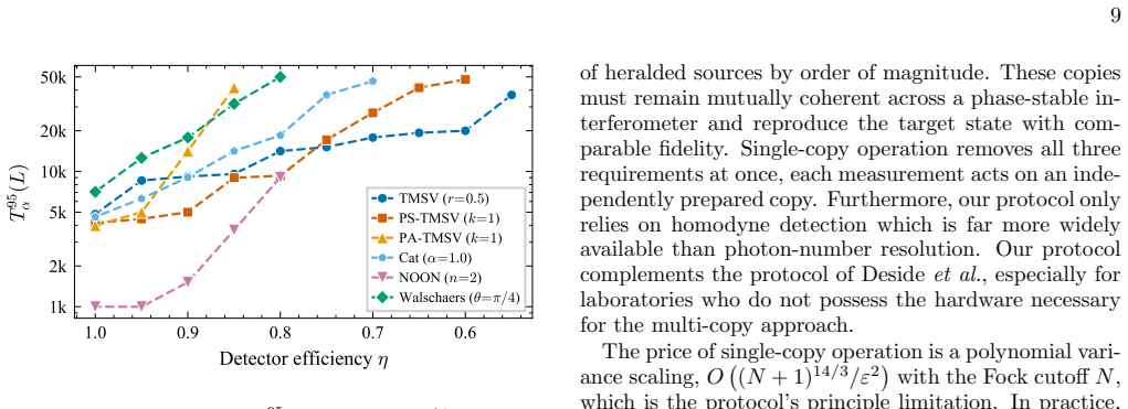
- The protocol applies equally to Gaussian and non-Gaussian states and reaches 95 % one-sided detection probability with 10³–10⁴ measurements when the mean photon number is approximately 2.
- Sample complexity remains polynomial in the Fock cutoff N, specifically O((N+1)^{14/3}/ε²).
- No photon-number-resolving detectors or multi-copy interferometry are required.
Where Pith is reading between the lines
- The randomization step is compatible with standard homodyne setups in which the local-oscillator phase is swept or chosen randomly across shots.
- The same estimator construction could be adapted to account for known detector inefficiency once the inefficiency model is folded into the moment definitions.
- Because the scaling is polynomial in N, modest improvements in measurement rate or parallel homodyne channels could bring higher-photon-number states within reach.
Load-bearing premise
Homodyne quadrature measurements can be performed in a sufficiently randomized fashion so that their statistics converge to the required partial-transpose moments without additional state-dependent corrections or unmodeled detector inefficiencies.
What would settle it
An experiment in which the homodyne-derived estimates of p2 and p3 deviate from the true partial-transpose moments by more than the claimed additive error for a state whose exact moments are known, or in which the empirical detection rate for a known entangled non-Gaussian state falls below 95 % at the predicted sample size.
Figures


read the original abstract
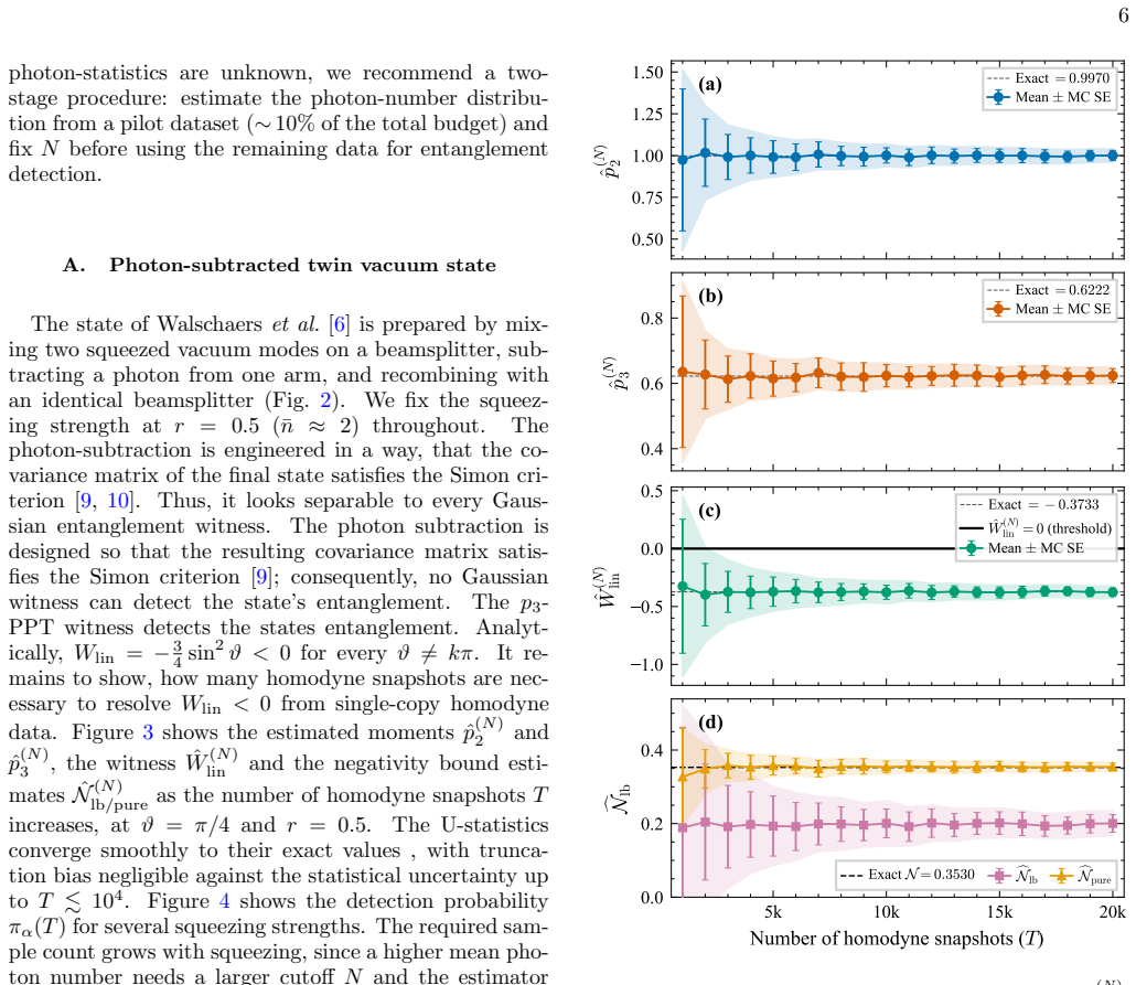
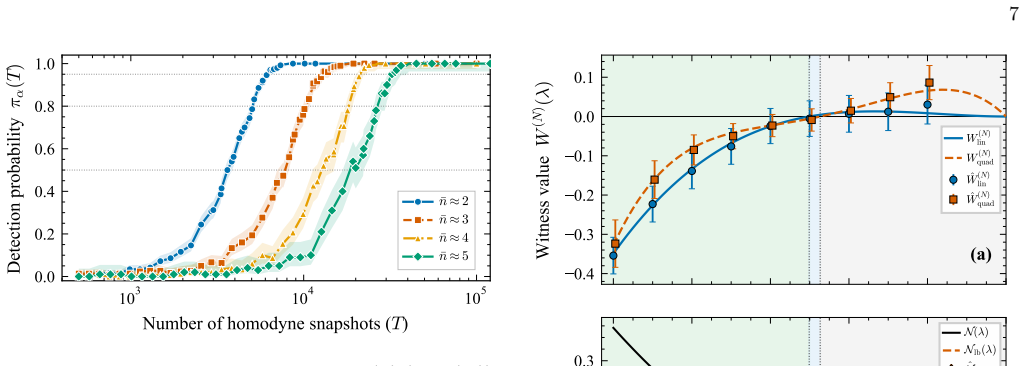
The entanglement of Gaussian continuous-variable (CV) states is fully determined by the state's second moments. In contrast, some entangled non-Gaussian states evade every second-moment criterion, and non-Gaussian entanglement detection remains an experimental challenge. The $p_3$-PPT criterion detects entanglement using moments of the partial transpose of the density matrix. This criterion was recently extended to CV systems using photon-number-resolving detectors and multi-copy interferometry; here we introduce a single-copy homodyne protocol that detects bipartite CV entanglement via the same criterion. Unbiased U-statistic estimators for the partial-transpose moments $p_2$ and $p_3$ are constructed directly from randomized homodyne data and used to evaluate the $p_3$-PPT entanglement witnesses: a linear one for detection, and a quadratic one whose violation yields a dimension-free lower bound on the entanglement negativity. The protocol estimates $p_2$ and $p_3$ up to additive error $\varepsilon$ at Fock cutoff $N$ from $O((N+1)^{14/3}/\varepsilon^2)$ measurements at fixed confidence. We demonstrate the protocol on six families of Gaussian and non-Gaussian states, reaching $95\%$ empirical one-sided detection probability from $\sim 10^3$ to $10^4$ homodyne measurements for states with $\bar{n} \approx 2$, placing non-Gaussian entanglement detection within reach of current homodyne experiments.
Editorial analysis
A structured set of objections, weighed in public.
Referee Report
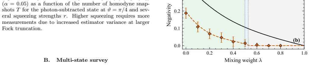
Summary. The paper claims to introduce a single-copy homodyne protocol for detecting bipartite continuous-variable entanglement via the p3-PPT criterion. It constructs unbiased U-statistic estimators for the partial-transpose moments p2 and p3 directly from randomized homodyne data, evaluates both a linear witness for detection and a quadratic witness yielding a dimension-free negativity lower bound, derives a sample complexity of O((N+1)^{14/3}/ε²) measurements to achieve additive error ε at Fock cutoff N, and demonstrates empirical performance on six families of states with ~10^3–10^4 measurements reaching 95% one-sided detection probability for states with mean photon number ≈2.
Significance. If the unbiasedness of the U-statistics is rigorously established and free of systematic offsets, the result would be significant for bringing non-Gaussian CV entanglement detection within reach of existing homodyne setups, extending the p3-PPT criterion beyond photon-number-resolving or multi-copy methods while also supplying an explicit negativity bound.
major comments (1)
- [Abstract / protocol construction] Abstract / protocol construction: the claim that the U-statistics are exactly unbiased for the PT moments p2 and p3 requires an explicit derivation showing that the joint statistics of randomized single-mode homodyne quadratures on both subsystems reproduce the relevant operator expectations on the partially transposed density operator. Any mismatch from non-uniform phase sampling, finite-N truncation, or unmodeled loss would introduce systematic bias, invalidating both the linear detection test and the quadratic negativity bound; this is load-bearing for the central claim.
minor comments (1)
- The abstract refers to demonstrations on 'six families of Gaussian and non-Gaussian states' without naming the families or citing their definitions or parameter values.
Simulated Author's Rebuttal
We thank the referee for their careful reading and for identifying the central importance of rigorously establishing unbiasedness of the U-statistics. We address the single major comment below. The derivation is already present in the manuscript but we agree that additional explicit steps will improve clarity and have revised accordingly.
read point-by-point responses
-
Referee: [Abstract / protocol construction] Abstract / protocol construction: the claim that the U-statistics are exactly unbiased for the PT moments p2 and p3 requires an explicit derivation showing that the joint statistics of randomized single-mode homodyne quadratures on both subsystems reproduce the relevant operator expectations on the partially transposed density operator. Any mismatch from non-uniform phase sampling, finite-N truncation, or unmodeled loss would introduce systematic bias, invalidating both the linear detection test and the quadratic negativity bound; this is load-bearing for the central claim.
Authors: We agree that unbiasedness is load-bearing and thank the referee for requiring an explicit verification. Section III and Appendix B already contain the derivation: the U-statistic for p_k is the average over products of single-mode homodyne outcomes with random phases heta, heta' drawn uniformly from [0,2π). Because the characteristic function of a homodyne quadrature measurement exactly reproduces the Weyl operators and the partial transpose on mode B corresponds to a sign flip in the phase of the quadrature operators on B, the expectation value of each term equals the corresponding moment Tr[(( ho^{T_B})^{\otimes k} P)], where P is the appropriate permutation operator; hence the U-statistic is exactly unbiased for the PT moments. Uniform phase sampling is stated in the protocol definition and the finite-N truncation is handled by projecting onto the N-photon subspace before taking moments, with the sample-complexity bound explicitly depending on (N+1). Ideal homodyne (no loss) is assumed, as is standard; any unmodeled loss would indeed introduce bias, but this is an experimental calibration issue rather than a flaw in the estimator itself. To address the referee’s concern we have added a new subsection (III.C) that walks through the expectation calculation line-by-line and explicitly states the assumptions on phase sampling and truncation. revision: yes
Circularity Check
No circularity in derivation of homodyne U-statistic estimators for p3-PPT moments
full rationale
The paper constructs unbiased U-statistic estimators for partial-transpose moments p2 and p3 directly from randomized single-copy homodyne data and derives sample-complexity bounds O((N+1)^{14/3}/ε²). This construction and the resulting linear/quadratic witnesses are presented as independent of the input data fits or prior self-citations; the p3-PPT criterion itself is referenced as prior work without the new protocol reducing to a self-referential definition or fitted prediction. No quoted step equates a claimed prediction to its own inputs by construction.
Axiom & Free-Parameter Ledger
axioms (2)
- standard math U-statistics constructed from i.i.d. samples yield unbiased estimators of the corresponding population moments
- domain assumption Homodyne quadrature measurements can be randomized sufficiently to sample the required partial-transpose moment distributions
Reference graph
Works this paper leans on
-
[1]
Efficient computation.Define the single-mode shadow matricesA i :=ρ (i) A andB i :=ρ (i) B (each (N+1)× (N+1))
Order-2 kernel:ˆp 2 The kernel for the second PT-moment is h2(Xi, Xj) =g A(Xi, Xj)g B(Xi, Xj),(A1) where the single-mode factor is gM(Xi, Xj) = NX n,m=0 Fn,m(x(i) M , θ(i) M )F m,n(x(j) M , θ(j) M ) (A2) Sinceh 2 is already symmetric underi↔j(by cyclicity of the trace), the symmetrized kernel ˜h2 =h 2, and the U-statistic is ˆp2 = T 2 −1X i<j h2(Xi, Xj).(...
-
[2]
(7)]: h3(Xi, Xj, Xk) = Tr h ρ(i) AB⊗ρ(j) AB⊗ρ(k) AB ˆΠ(A) (123)⊗ˆΠ(B) (132) i
Order-3 kernel:ˆp 3 The kernel for the third PT-moment uses the opposite- chirality cyclic shift [Eq. (7)]: h3(Xi, Xj, Xk) = Tr h ρ(i) AB⊗ρ(j) AB⊗ρ(k) AB ˆΠ(A) (123)⊗ˆΠ(B) (132) i . (A7) Writing out the index contraction: h3(Xi, Xj, Xk) = X a1,a2,a3 b1,b2,b3 [Ai]a1,a2 [Bi]b1,b3 [Aj]a2,a3 [Bj]b2,b1 ×[A k]a3,a1 [Bk]b3,b2 = Tr[Ai Aj Ak] Tr[BT i BT j BT k ]. ...
-
[3]
The subsequent matrix operations (Tr[S 2], Tr[S3]) areO(N 6), subdomi- nant forT≫N 2
Computational complexity The bottleneck for both estimators is theO(T N 4) ac- cumulation ofS(A4): for each of theTsnapshots, the outer productA i ⊗B T i hasN 4 entries. The subsequent matrix operations (Tr[S 2], Tr[S3]) areO(N 6), subdomi- nant forT≫N 2. For the sample sizes and cutoffs in this paper (T≤ 5×10 4,N≤10), the total computation takes seconds ...
-
[4]
re- alistic
Then: (i)The negativity satisfies the cubic bound N(ρ)≥β ∗,(D1) whereβ ∗ is the smallest positive real root of g(u) =u 3 + 2p2 u2 +p 3 u+ (p 3 −p 2 2).(D2) 13 (ii)The negativity also satisfies the closed-form ratio- nal bound N(ρ)≥ p2 2 −p 3 p2 +p 3 + 1 4 .(D3) (iii)For pure states (p 2 = 1), the cubic factors as g(u) = (u+ 1)(u 2 +u+p 3 −1) and the bound...
-
[5]
Witness value of the linear witnessW lin, for different states under detector ineffeciency and homodyne phase jitter
Robustness to loss and phase jitter 15 0 50 100 150 200 250 300 350 Phase jitter σθ (mrad) T M SV (r = 0.3) W quad T M SV (r = 0.5) W quad 0 50 100 150 200 250 300 350 Phase jitter σθ (mrad) P S-T M SV (r = 0.5, k = 1) WlinW quad P S-T M SV (r = 0.5, k = 2) W lin Wquad 0 50 100 150 200 250 300 350 Phase jitter σθ (mrad) P A -T M SV (r = 0.3, k = 1) W lin ...
-
[6]
Lloyd and S
S. Lloyd and S. L. Braunstein, Quantum Computation over Continuous Variables, Phys. Rev. Let.82(1999)
1999
-
[7]
Mari and J
A. Mari and J. Eisert, Positive Wigner Functions Render Classical Simulation of Quantum Computation Efficient, Physical Review Letters109, 230503 (2012)
2012
-
[8]
Gottesman, A
D. Gottesman, A. Kitaev, and J. Preskill, Encoding a qubit in an oscillator, Phys. Rev. A64, 012310 (2001)
2001
-
[9]
Niset, J
J. Niset, J. Fiur´ aˇ sek, and N. J. Cerf, No-Go Theorem for Gaussian Quantum Error Correction, Physical Review Letters102, 120501 (2009)
2009
-
[10]
Entanglement Certification $-$ From Theory to Experiment
N. Friis, G. Vitagliano, M. Malik, and M. Huber, Entan- glement certification from theory to experiment, Nature Rev. Phys.1, 72 (2018), arXiv:1906.10929 [quant-ph]
work page internal anchor Pith review Pith/arXiv arXiv 2018
-
[11]
M. Walschaers, Non-Gaussian Quantum States and Where to Find Them, PRX Quantum2, 030204 (2021), 2104.12596
-
[12]
R. F. Werner and M. M. Wolf, Bound entangled gaussian states, Phys. Rev. Lett.86, 3658 (2001)
2001
-
[13]
L.-M. Duan, G. Giedke, J. I. Cirac, and P. Zoller, Insep- arability criterion for continuous variable systems, Phys. Rev. Lett.84, 2722 (2000), quant-ph/9908056
work page internal anchor Pith review Pith/arXiv arXiv 2000
-
[14]
Peres-Horodecki separability criterion for continuous variable systems
R. Simon, Peres-Horodecki separability criterion for con- tinuous variable systems, Phys. Rev. Lett.84, 2726 (2000), quant-ph/9909044
work page internal anchor Pith review Pith/arXiv arXiv 2000
-
[15]
Walschaers, C
M. Walschaers, C. Fabre, V. Parigi, and N. Treps, En- tanglement and Wigner Function Negativity of Multi- mode Non-Gaussian States, Phys. Rev. Lett.119, 183601 (2017)
2017
-
[16]
Saboia, F
A. Saboia, F. Toscano, and S. P. Walborn, Family of continuous-variable entanglement criteria using general entropy functions, Phys. Rev. A83, 032307 (2011)
2011
-
[17]
Shchukin and W
E. Shchukin and W. Vogel, Inseparability Criteria for Continuous Bipartite Quantum States, Phys. Rev. Lett. 95, 230502 (2005)
2005
- [18]
-
[19]
Elben, R
A. Elben, R. Kueng, H.-Y. R. Huang, R. Van Bij- nen, C. Kokail, M. Dalmonte, P. Calabrese, B. Kraus, J. Preskill, P. Zoller, and B. Vermersch, Mixed-State Entanglement from Local Randomized Measurements, Phys. Rev. Lett.125, 200501 ()
-
[20]
The randomized measurement toolbox
A. Elben, S. T. Flammia, H.-Y. Huang, R. Kueng, J. Preskill, B. Vermersch, and P. Zoller, The randomized measurement toolbox, Nat Rev Phys5, 9 (), 2203.11374
- [21]
-
[22]
Deside, T
S. Deside, T. Haas, and N. J. Cerf, Detecting strongly non-gaussian entanglement, Phys. Rev. Res. , (2026)
2026
-
[23]
P. Cie´ sli´ nski, S. Imai, J. Dziewior, O. G¨ uhne, L. Knips, W. Laskowski, J. Meinecke, T. Paterek, and T. V´ ertesi, Analysing quantum systems with randomised measure- ments, Physics Reports1095, 1 (2024), 2307.01251
-
[24]
Huang, R
H.-Y. Huang, R. Kueng, and J. Preskill, Predicting many properties of a quantum system from very few measure- ments, Nature Physics16, 1050–1057 (2020)
2020
-
[25]
Becker, N
S. Becker, N. Datta, L. Lami, and C. Rouze, Classical Shadow Tomography for Continuous Variables Quantum Systems, IEEE Trans. Inform. Theory70, 3427 (2024)
2024
-
[26]
Gandhari, V
S. Gandhari, V. V. Albert, T. Gerrits, J. M. Taylor, and M. J. Gullans, Precision Bounds on Continuous-Variable State Tomography Using Classical Shadows, PRX Quan- tum5, 010346 (2024)
2024
-
[27]
Christandl and R
M. Christandl and R. Renner, Reliable quantum state tomography, Phys. Rev. Lett.109, 120403 (2012)
2012
-
[28]
A. I. Lvovsky and M. G. Raymer, Continuous-variable optical quantum-state tomography, Rev. Mod. Phys.81, 299 (2009)
2009
-
[29]
Peres, Separability Criterion for Density Matrices, Phys
A. Peres, Separability Criterion for Density Matrices, Phys. Rev. Lett.77, 1413 (1996)
1996
-
[30]
Leonhardt,Measuring the Quantum State of Light (Cambridge University Press, Cambridge, 1997)
U. Leonhardt,Measuring the Quantum State of Light (Cambridge University Press, Cambridge, 1997)
1997
-
[31]
An invitation to quantum tomography
L. Artiles, R. Gill, and M. Guta, An invitation to quan- tum tomography, Journal of the Royal Statistical Society. Series B67, 109 (2005), arXiv:quant-ph/0303020
work page internal anchor Pith review Pith/arXiv arXiv 2005
-
[32]
Richter, Realistic pattern functions for optical homo- dyne tomography and determination of specific expecta- tion values, Physical Review A61, 063819 (2000)
Th. Richter, Realistic pattern functions for optical homo- dyne tomography and determination of specific expecta- tion values, Physical Review A61, 063819 (2000)
2000
-
[33]
A. K. Ekert, C. M. Alves, D. K. L. Oi, M. Horodecki, P. Horodecki, and L. C. Kwek, Direct Estimations of Lin- ear and Nonlinear Functionals of a Quantum State, Phys. Rev. Lett.88, 217901 (2002)
2002
-
[34]
Y. Zhou, P. Zeng, and Z. Liu, Single-Copies Estimation of Entanglement Negativity, Phys. Rev. Lett.125, 200502 (2020)
2020
-
[35]
Hoeffding, Probability inequalities for sums of bounded random variables, Journal of the American Sta- tistical Association58, 13 (1963)
W. Hoeffding, Probability inequalities for sums of bounded random variables, Journal of the American Sta- tistical Association58, 13 (1963)
1963
-
[36]
R. J. Serfling,Approximation Theorems of Mathematical Statistics, Wiley Series in Probability and Mathematical Statistics (John Wiley & Sons, New York, 1980)
1980
-
[37]
A. J. Lee,U-Statistics: Theory and Practice(Marcel Dekker, New York, 1990)
1990
-
[38]
Hoeffding, A Class of Statistics with Asymptoti- cally Normal Distribution, The Annals of Mathematical Statistics19, 293 (1948)
W. Hoeffding, A Class of Statistics with Asymptoti- cally Normal Distribution, The Annals of Mathematical Statistics19, 293 (1948)
1948
-
[39]
Vidal and R
G. Vidal and R. F. Werner, Computable measure of en- tanglement, Phys. Rev. A65, 032314 (2002)
2002
-
[40]
M. B. Plenio, Logarithmic negativity: A full entangle- ment monotone that is not convex, Phys. Rev. Lett.95, 090503 (2005)
2005
-
[41]
H. A. Carteret, Estimating the entanglement negativity from low-order moments of the partially transposed den- sity matrix (2017), arXiv:1605.08751 [quant-ph]
work page internal anchor Pith review Pith/arXiv arXiv 2017
-
[42]
Bartkiewicz, J
K. Bartkiewicz, J. c. v. Beran, K. Lemr, M. Norek, and A. Miranowicz, Quantifying entanglement of a two- qubit system via measurable and invariant moments of its partially transposed density matrix, Phys. Rev. A91, 022323 (2015)
2015
-
[43]
Rana, Negative eigenvalues of partial transposition of arbitrary bipartite states, Phys
S. Rana, Negative eigenvalues of partial transposition of arbitrary bipartite states, Phys. Rev. A87, 054301 (2013)
2013
-
[44]
Code will be made available in a public repository upon publication
-
[45]
J. N. Arvesen, Jackknifing U-statistics, The Annals of Mathematical Statistics40, 2076 (1969)
2076
-
[46]
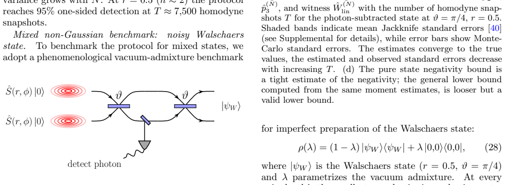
Continuous-variable teleportation improvement by photon subtraction via conditional measurement
T. Opatrn´ y, G. Kurizki, and D.-G. Welsch, Improvement on teleportation of continuous variables by photon sub- traction via conditional measurement, Physical Review A61, 032302 (2000), arXiv:quant-ph/9907048. 17
work page internal anchor Pith review Pith/arXiv arXiv 2000
-
[47]
Enhancing quantum entanglement by photon addition and subtraction
C. Navarrete-Benlloch, R. Garc´ ıa-Patr´ on, J. H. Shapiro, and N. J. Cerf, Enhancing quantum entanglement by photon addition and subtraction, Physical Review A86, 012328 (2012), arXiv:1201.4120 [quant-ph]
work page internal anchor Pith review Pith/arXiv arXiv 2012
-
[48]
A. N. Boto, P. Kok, D. S. Abrams, S. L. Braunstein, C. P. Williams, and J. P. Dowling, Quantum interfero- metric optical lithography: Exploiting entanglement to beat the diffraction limit, Physical Review Letters85, 2733 (2000)
2000
-
[49]
B. C. Sanders, Review of entangled coherent states, Jour- nal of Physics A: Mathematical and Theoretical45, 244002 (2012), arXiv:1112.1778 [quant-ph]
work page internal anchor Pith review Pith/arXiv arXiv 2012
-
[50]
Kumar, E
R. Kumar, E. Barrios, A. MacRae, E. Cairns, E. Hunt- ington, and A. Lvovsky, Versatile wideband balanced de- tector for quantum optical homodyne tomography, Op- tics Communications285, 5259 (2012)
2012
-
[51]
Y.-D. Wu, Y. Zhu, G. Chiribella, and N. Liu, Efficient learning of continuous-variable quantum states, Physical Review Research6, 10.1103/physrevresearch.6.033280 (2024)
-
[52]
F. A. Mele, A. A. Mele, L. Bittel, J. Eisert, V. Giovan- netti, L. Lami, L. Leone, and S. F. E. Oliviero, Learning quantum states of continuous-variable systems, Nature Physics21, 2002–2008 (2025)
2002
-
[53]
F. A. Mele, Advances in quantum learning theory with bosonic systems (2026), arXiv:2605.08082 [quant-ph]
work page internal anchor Pith review Pith/arXiv arXiv 2026
-
[54]
Killoran, J
N. Killoran, J. Izaac, N. Quesada, V. Bergholm, M. Amy, and C. Weedbrook, Strawberry fields: A software plat- form for photonic quantum computing, Quantum3, 129 (2019)
2019
-
[55]
T. R. Bromley, J. M. Arrazola, S. Jahangiri, J. Izaac, N. Quesada, A. D. Gran, M. Schuld, J. Swinarton, Z. Zabaneh, and N. Killoran, Applications of near-term photonic quantum computers: software and algorithms, Quantum Science and Technology5, 034010 (2020). 18 Supplemental Material: Detecting non-Gaussian entanglement from single-copy homodyne measureme...
2020
-
[56]
[25], which evaluatesF n,m(x, θ) through stable recur- rence relations for the harmonic-oscillator wave functions
Ideal pattern functions For completeness, we summarize the numerical recipe of Ref. [25], which evaluatesF n,m(x, θ) through stable recur- rence relations for the harmonic-oscillator wave functions. The amplitudef n,m(x) is obtained forn≥mfrom fn,m(x) = 2xψm(x)φn(x)− p 2(m+ 1)ψ m+1(x)φn(x)− p 2(n+ 1)ψ m(x)φn+1(x).(S2) Hereψ m(x) are the regular harmonic-o...
-
[57]
Instead, we need to use pattern functions that depend on the detector efficiencyF n,m(x, θ;η)
Realistic pattern functions If the detector efficiency isη <1, theidealpattern functionsF n,m(x, θ) are no longer unbiased. Instead, we need to use pattern functions that depend on the detector efficiencyF n,m(x, θ;η). The main result of Ref.[27] shows how to expressF n,m(x, θ;η) as a finite sum of ideal pattern functionsF n,m(x, θ): Fn,m(x, θ;η) = r η 2η...
-
[58]
, Xk)|X 1,
Hoeffding decomposition The variance of an order-kU-statistic with symmetric kernel ˜hk admits the exact decomposition [31, 32] Var(ˆpk) = kX c=1 k c 2 σ2 k,cT c ,(S1) where the Hoeffding components are σ2 k,c = Var E[˜hk(X1, . . . , Xk)|X 1, . . . , Xc] (S2) (the variance of the conditional expectation givencof thekarguments, averaged over the remainingk...
-
[59]
First Hoeffding projections The leading variance components are determined by thefirst Hoeffding projections: G2(X) =E X ′[h2(X, X ′)|X]−p 2 = Tr ˆΣTB N (X)ρ TB −p 2,(S5) G3(X) =E X ′,X ′′[h3(X, X ′, X′′)|X]−p 3 = Tr ˆΣTB N (X) (ρTB)2 −p 3,(S6) where ˆΣTB N (X) =ρ (X) A ⊗(ρ (X) B )T is the partial-transposed single-shot shadow. Proof of(S5)and(S6).The ord...
-
[60]
Entry-wise control of the snapshot second moment The state-independent variance bound quoted in the main text is obtained most directly by the pointwise Hilbert– Schmidt argument of Sec. SV. What that argument does not provide, and what the state-dependentgeometric-decay analysis of Sec. SIV 4 below requires, is a bound on the snapshot second-moment matri...
-
[61]
State-dependent bounds under geometric decay For states satisfying the geometric Fock-decay condition |[ρTB](nk),(ml)| ≤C ρ r(n+k+m+l)/2, r <1,(GD) 24 (which holds for TMSV withC ρ = sech2rs andr= tanhr s, and for photon-subtracted states with the samerand modifiedC ρ), the leading variance components are bounded independently ofN. Theorem SIV.2 (N-indepe...
-
[62]
The quadratic witness, in contrast, involves the square of ˆp 2 and acquires a finite-sample bias, which we quantify and correct here
Bias correction of the quadratic witness The linear witness estimator ˆWlin = ˆp3 −(3ˆp2 −1)/2 is a linear combination of unbiased U-statistics and is therefore exactly unbiased. The quadratic witness, in contrast, involves the square of ˆp 2 and acquires a finite-sample bias, which we quantify and correct here. 25 a. Exact bias identity The quadratic wit...
-
[63]
They use the same leave-one-out variance estimate as the bias correction of Sec
Jackknife standard errors The shaded uncertainty bands in the figures of the main text are jackknife (influence-function) standard errors [40]. They use the same leave-one-out variance estimate as the bias correction of Sec. SIV 5 b, now applied to each estimator in turn. For the order-kU-statistic ˆpk, the empirical first Hoeffding projection ˆGk(Xi) is ...
-
[64]
bound the Hilbert–Schmidt norm of a single-mode snapshot (Sec. SV 1)
-
[65]
tensorize to the bipartite snapshot that the protocol actually measures (Sec. SV 2)
-
[66]
SIV to obtain state-independent variances for the moment estimators and both witnesses (Sec
feed this pointwise bound into the exact Hoeffding variance formulas of Sec. SIV to obtain state-independent variances for the moment estimators and both witnesses (Sec. SV 3)
-
[67]
SV 4 and SV 5)
apply Chebyshev’s inequality to convert the variances into the sample-complexity bound (Secs. SV 4 and SV 5). Throughout,d=N+ 1 denotes the local Hilbert-space dimension at Fock cutoffN. All bounds in this section are state-independent and hold for any bipartite state with finite mean photon number ¯n <∞
-
[68]
One-mode snapshot norm bound Fix a single modeMwith Fock cutoffN. A homodyne measurement with outcomexat phaseθproduces the shadow matrixρ M(x, θ) =PN n,m=0 Fnm(x, θ)|n⟩⟨m|(S1), whose Hilbert–Schmidt norm squared is ρM(x, θ) 2 2 = NX n,m=0 |Fnm(x, θ)|2 = NX n,m=0 fnm(x)2.(S1) The phase entersF nm(x, θ) only through a unit-modulus factor, so|F nm(x, θ)|=|f...
-
[69]
The partial-transposed bipartite shadow from a single measurement round is ˆΣTB N (X) =ρ A(xA, θA)⊗(ρ B(xB, θB))T
Bipartite tensorization The one-mode bound carries over to the bipartite case at once, because the snapshot the protocol actually measures is a tensor product of two single-mode shadows. The partial-transposed bipartite shadow from a single measurement round is ˆΣTB N (X) =ρ A(xA, θA)⊗(ρ B(xB, θB))T . As in Sec. SIV, we writez(X) = vec( ˆΣTB N (X)) for th...
-
[70]
Variance bounds forˆp 2 andˆp3 We now insert the pointwise norm bound into the exact U-statistic variance formulas from the Hoeffding decom- position (Sec. SIV). We first note that the order-kkernels themselves obey pointwise bounds inherited directly from the snapshot Hilbert–Schmidt norm. Lemma SV.5 (Kernel bounds).For any measurement outcomesX 1, . . ....
-
[71]
Proof.—By Chebyshev’s inequality and (S12): Pr(|ˆp 2 −p 2|> ε)≤Var(ˆp 2)/ε2 ≤16C 2 pf (N+ 1) 14/3/(T ε2)
Sample complexity Theorem SV.6 (State-independent sample complexity).For any bipartite stateρwith¯n <∞and Fock cutoffN, the U-statistic estimatorsˆp 2,ˆp3, and the witnesses ˆWlin, ˆWquad can be estimated to additive accuracyεwith probability≥1−δusing T=O (N+ 1) 14/3 δ ε2 (S22) samples, via Chebyshev’s inequality. Proof.—By Chebyshev’s inequality and (S12...
-
[72]
Non-asymptotic constants and certification rules The variance bounds derived so far carryO(T −2) remainders from the higher Hoeffding components, hidden inside theO(·) notation. This subsection discharges those remainders rigorously and pins down the explicit constants K2 = 32 andK 3 = 108, together with the certification constantsC W , exactly as quoted ...
-
[73]
Discussion The exponent 7/3 in Lemma SV.1 is attained near the Airy transition region, where the pattern functions are maximally oscillatory. Within the present argument it cannot be improved, because the bound treats every measure- ment outcome in the worst case, through theℓ ∞ norm of the pattern functions, and so discards all information about how the ...
-
[74]
Negativity under local compression For any positive trace-classτ(not necessarily normalized), define itsunnormalized negativity N∗(τ) := Tr (τ TB)− = ∥τ TB ∥1 −Tr[τ] 2 .(S1) When Tr[τ] = 1, this is the usual negativity. Physically, projecting onto a finite Fock window discards weight from ρTB and can only shrink the negative part, so the truncated negativ...
-
[75]
In particular,Tr[(τ TB)3]≥ −(t/2) Tr[(τ TB)2]
Spectral range for subnormalized partial transposes Lemma SVI.2 (Subnormalized spectral range).Ifτ≥0withTr[τ] =t, then every eigenvalue ofτ TB lies in [−t/2, t]. In particular,Tr[(τ TB)3]≥ −(t/2) Tr[(τ TB)2]. Proof.—Define the normalized stateσ=τ /t. By Proposition SIII.1,− 1 2 I≤σ TB ≤I. Multiplying bytgives − t 2 I≤τ TB ≤tI. The scalar inequalityx 3 ≥ −...
-
[76]
Truncated negativity bounds Writeq k =p (N) k = Tr[(ρTB N )k] for brevity, withq 1 =t N. Define thetruncated third-order deficit ∆N :=q 2 2 −t N q3 = p(N) 2 2 −t N p(N) 3 .(S3) Note that this is the Hankel determinant det tN q2 q2 q3 of the subnormalized moment sequence, not the deficitq 2 2 −q 3 used by the normalized witness. Theorem SVI.3 (Truncated ne...
-
[77]
Pure-state specialization For a pure input state|ψ⟩, the projected operatorρ N =P N |ψ⟩⟨ψ|P N =| ˜ψ⟩⟨ ˜ψ|is a rank-one operator of norm ⟨ ˜ψ| ˜ψ⟩=t N, soq 2 = Tr[ρ2 N] =t 2 N using the invariance of the Hilbert–Schmidt norm under partial transposition. Substitutingq 2 =t 2 N into the cubic (S5) factors it as tN u3 + 2t2 N u2 +q 3u+t N q3 −t 4 N = (u+t N) ...
discussion (0)
Sign in with ORCID, Apple, or X to comment. Anyone can read and Pith papers without signing in.