Causal effect on the number of life years lost due to a specific event: Average treatment effect and variable importance

Simon Christoffer Ziersen; Torben Martinussen

REVIEW 2 major objections 5 minor 9 references

Causal effect on the number of life years lost due to a specific event: Average treatment effect and variable importance

T0 review · 2 major / 5 minor · reviewed 2026-08-09 · deepseek-v4-flash

Challenge this review Re-run · record.json Download PDF Read on arXiv ↗

Pith's one-line read The paper derives efficient, machine-learning-based estimators for the causal effect on the number of life years lost due to a specific event, with valid inference under flexible nuisance estimation.

desk verdict Solid, conditional semiparametric theory for a useful life-years-lost estimand, but the machine-learning bridge rests on unverified rate conditions and the simulation does not close that gap. read the letter →

arxiv 2502.00120 v1 pith:MSEEKXX7 submitted 2025-01-31 stat.ME

Simon Christoffer Ziersen , Torben Martinussen This is my paper · ORCID

classification stat.ME MSC 62D2062N0162G20

keywords Causalinferencenumberoflifeyearslostdebiasedlearningheterogeneitynonparametricsurvivaldatacompetingrisksvariableimportancemeasure

verification ladder T0 review T1 audit T2 compute T3 formal

The pith

A machine-rendered reading of the paper's core claim, the machinery that carries it, and where it could break.

The reading

This paper introduces a causal version of the number of life years lost due to a specific event, an estimand that reports how much time before a given horizon is lost because a particular cause of death occurs. The authors show that the average treatment effect on this estimand, as well as a variable importance measure for whether the treatment effect changes with a covariate, is identified under standard causal assumptions with competing risks. They derive efficient influence functions and build cross-fitted one-step estimators that remain asymptotically normal when the nuisance functions are estimated with flexible machine learning. The result matters because it puts a clinically interpretable, time-scale treatment effect on the same footing as modern debiased causal inference, and the accompanying heterogeneity test gives a scale-free way to identify which covariates drive differential treatment response.

What carries the argument

The engine is the efficient influence function (EIF) of each target parameter combined with K-fold cross-fitting of a one-step estimator. For the ATE, the uncentered EIF is $\phi_j(\nu)(O)=\tau_j(X)+\{1(A=1)/\pi(1|X)-1(A=0)/\pi(0|X)\}\sum_{i=1}^2\int_0^{t^*}H_{ij}(s,t^*|A,X)/S_C(s|A,X)\,dM_i(s|A,X)$, where $H_{ij}$ is an integral of cumulative-incidence differences and $M_i$ are the cause-specific martingales; for the importance parameter, the EIF is built from the product of this centered ATE influence function with the covariate residual $X_l-E(X_l|X_{-l})$, normalized by the variance denominator. Cross-fitting—splitting the data into $K$ folds and evaluating each fold's score at nuisance estimates from the other folds—controls the empirical process term, so the remaining work is to bound a second-order remainder term and impose $n^{-1/4}$ convergence rates for the meta-learned regressions.

What would settle it

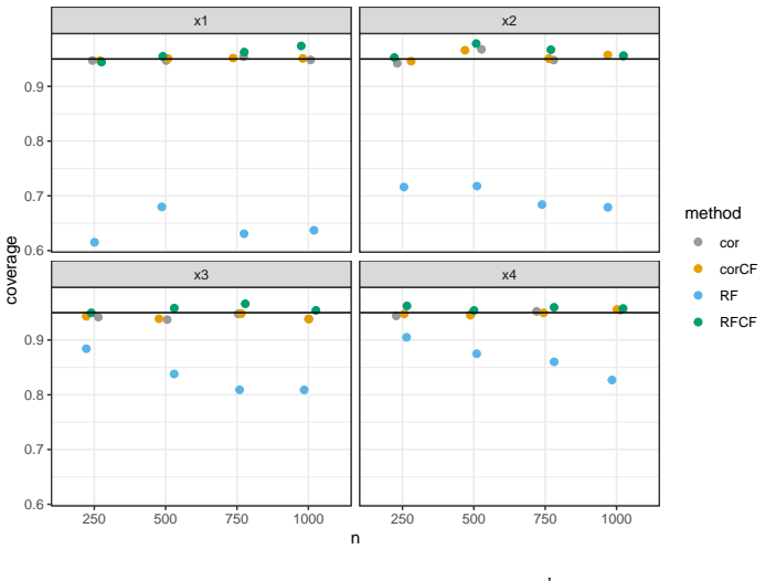
Simulate data with a known true ATE and generate it with the cause-specific hazards as in Section 5, then estimate the ATE with the proposed cross-fitted estimator using random survival forests as nuisance learners and compute the empirical coverage of the confidence interval at increasing sample sizes; if coverage does not approach 0.95 and bias does not decay at $n^{-1/2}$ as $n$ grows, the remainder condition B3 is violated for that learner and the theorem's conclusion fails for that data process.

Watch

Extended reading notes

Core claim

The central claim is that the average treatment effect on the number of life years lost due to a specific event, defined as $\psi_j(P)=E\{L_j(0,t^*|1,X)-L_j(0,t^*|0,X)\}$ with $L_j$ the integrated cumulative incidence, is estimable with a cross-fitted one-step estimator that is asymptotically linear with influence function $\tilde{\psi}_{\psi_j}$ under Assumption B. For the variable importance measure $\Omega_l^j$, defined as the best partially linear projection of the conditional average treatment effect onto covariate $X_l$, the paper proves an analogous result with influence function $\tilde{\psi}_{\Omega_l^j}$, and gives an asymptotically standard normal test statistic for $H_0:\Omega_l^j=0$. The proofs identify the efficient influence functions explicitly, including the inverse-propensity-weighted martingale representation, and show that cross-fitting removes the Donsker-class requirement, leaving only high-level convergence-rate conditions on the nuisance estimators. In simulations, random-forest nuisance estimation with cross-fitting achieves near-nominal coverage, and the application to antidepressant registry data illustrates how the new estimand changes the interpretation from probability differences to days of healthy life lost.

Load-bearing premise

All the stated guarantees depend on unverifiable high-level rate conditions: the ATE needs the nuisance remainder to vanish at root-n speed, and the heterogeneity test additionally needs the meta-learned regression of treatment-effect estimates onto other covariates to be accurate to within $n^{-1/4}$; if the chosen machine learners do not meet these rates in a given data-generating process, the asymptotic normality and standard errors do not follow.

Editorial extensions

If this is right

Applied researchers can use random survival forests or other flexible learners for the cause-specific hazards, censoring, and propensity score without giving up valid confidence intervals, provided the high-level rate conditions hold; the simulation study shows near-nominal coverage for the cross-fitted version.
The test based on $T_{ST}^l$ is asymptotically standard normal under the null $\Omega_l^j=0$, so it provides a scale-free, p-value-based ranking of covariates by their contribution to treatment-effect heterogeneity in the presence of competing risks.
Because the estimand is defined directly on the time scale of the data, the ATE is reported in units such as days of healthy life lost, which is more directly interpretable to clinicians than differences in cumulative incidence probabilities.
The estimator avoids the need for correctly specified parametric models for the conditional average treatment effect or the censoring distribution, unlike pseudo-observation-based competitors.
The framework applies to any specified competing event, and the paper notes that recomputing the importance ranking with event and competing event swapped can reveal whether an apparent effect on one cause is driven by the other.

Reading between the lines

Editorial extensions of the paper, not claims the author makes directly.

Beyond the paper's claims, the explicit form of the remainder term suggests the ATE estimator may be doubly robust—consistent if either the hazard pair or the propensity/censoring pair is correctly specified—which would be worth testing under model misspecification.
Beyond the paper's claims, the method could be turned into a functional estimator by letting the horizon $t^*$ vary and reporting $\hat{\psi}_j^{CF}(t^*)$ as a curve, providing a treatment-effect trajectory rather than a single summary.
Beyond the paper's claims, because the importance parameter is scale-dependent, an explicit recommendation would be to standardize covariates before computing $\Omega_l^j$ when comparing importance across variables measured in different units, or to rely solely on the p-value ranking as the application does.
Beyond the paper's claims, pairing the EIF-based estimator with a stacking ensemble that explicitly targets the $n^{-1/4}$ rate for the meta-learned CATE regression might make the asymptotic guarantees more robust in small samples than a single black-box learner.

Share X Bluesky LinkedIn Reddit HN

Editorial analysis

A structured set of objections, weighed in public.

Desk editor's note, referee report, and a circularity audit.

Desk Editor's Note

read the letter

This is a competent methods paper. The estimand itself has been around since Andersen (2013), but the efficient cross-fitted estimator with flexible nuisance estimation is new, and so is the extension of the best partially linear projection variable importance to competing risks. The influence function derivations are careful and standard, and the explicit remainder representation in Lemma C.1 is a real strength. The simulation study is honest: it compares correctly specified parametric nuisance estimators with random forests, with and without cross-fitting, and the RFCF results show good coverage in that setup. That is genuine evidence of practical behavior, and the paper deserves credit for reporting both the failures of non-cross-fitted RF and the overcoverage in the cross-fitted version.

The soft spot is exactly what the stress-test note says. Assumption B3 is the load-bearing condition for the ATE theorem, and the authors themselves admit it is not established for Breslow-type or random survival forest estimators. Theorem 2 adds an n^{-1/4} rate for the meta-learned regression of CATE estimates onto X_{-l}, a rate they say is generally unknown. The simulations show finite-sample coverage around 0.95-0.97 for RFCF in one DGP, but that cannot establish a rate condition. So the claims of being 'model-agnostic' and 'efficient' are stronger than what is actually proved. The theorems are logically valid conditionally; the issue is an unsupported bridge between abstract assumptions and the recommended implementation, not an internal contradiction. A careful referee should ask the authors to either verify B3 for their RSF implementation under additional structural assumptions, or temper the practical claims accordingly.

Minor issues: no code or data are provided, and the consistency of the variance estimator relies on a self-cited lemma from their earlier paper. That is acceptable if the cited result is correct, but it would strengthen the paper to state or prove it in the appendix.

Who it is for: biostatisticians and methodological statisticians working on causal inference with competing risks, especially those interested in time-scale estimands and heterogeneous treatment effects. It deserves a serious referee. My recommendation: send it to peer review, and push for a revision that confronts the gap between the rate conditions and the recommended machine learning procedures.

Referee Report

2 major / 5 minor

Summary. The paper introduces causal estimands for the expected number of life-years lost due to a specific competing event within a fixed horizon, defines the average treatment effect (ATE) and a variable importance measure based on the best partially linear projection of the CATE, derives their efficient influence functions in the nonparametric model, and constructs cross-fitted one-step estimators with machine-learned nuisance parameters. Theorem 1 and Theorem 2 establish asymptotic linearity under high-level nuisance conditions, and a simulation study plus an application to Danish register data on antidepressants illustrate the methods.

Significance. The estimand is interpretable on the original time scale and complements cumulative-incidence-based effect measures, which is a genuine practical advantage. The EIF derivations are detailed and the remainder-term representation in Lemma C.1 is explicit, making the theoretical framework reproducible. The variable importance extension with a formal heterogeneity test is valuable for applied work. The principal weakness is that the advertised model-agnostic guarantees depend on high-level rate conditions, especially Assumption B3 and Theorem 2(ii), that are not shown to hold for the random forest implementations recommended in the simulation and application.

major comments (2)

[§4.1 (Assumption B3), §5, §7] The paper's central claim that the estimators are 'model-agnostic, asymptotically normal, and efficient' for machine-learned nuisance parameters is not established for the recommended implementations. Assumption B3 requires an o_p(n^{-1/2}) remainder term, and the text itself states (Section 4.1 and Section 7) that this is difficult to prove without absolute continuity of the cumulative hazard estimators and is unclear for random survival forests. The simulation results in Section 5 cannot verify an asymptotic rate condition; finite-sample coverage in a single DGP is not evidence that B3 holds. To support the abstract's claim, the authors should either prove B3 for a concrete class of data-adaptive estimators or provide verifiable sufficient conditions, or restrict the theoretical claims to estimators satisfying the high-level assumptions and label the random forest results as an empirical illustration rather than a confirmation.
[§4.2, Theorem 2, condition (ii)] Theorem 2's asymptotic normality for the variable importance estimator assumes that the meta-learned regression of the CATE estimates onto X_{-l} achieves ||\hat τ_l - τ_l|| = o_p(n^{-1/4}). The authors acknowledge in Section 4.2 that convergence rates for this step are 'generally less known.' Since the p-values in Section 6 are obtained from Theorem 2, the inference guarantee for the recommended procedure is incomplete. Please provide sufficient conditions for the meta-learner that yield condition (ii), or explicitly state that the inference is conditional on an unverified rate.

minor comments (5)

[Abstract and references] The abstract cites 'Andersen et al. (2013)' but the reference list entry is a single-author paper (Andersen, 2013); please correct the citation.
[Throughout] The drug name is misspelled as 'Setraline' in Sections 1 and 6; the correct spelling is 'Sertraline'. Also fix 'its standard' to 'it is standard' (Section 1), 'abbreveations' to 'abbreviations' (Table 1 caption), and 'on the marked' to 'on the market' and 'we constrict ourselves' to 'we restrict ourselves' (Section 6).
[§4.2] The displayed formula for \hat σ^{2,CF}_{Ω^l_j} is difficult to parse because of the nested parentheses; add explicit brackets or define an intermediate quantity for clarity.
[§3] The notation for the counterfactual event time T^a_j is introduced but the construction Y^a_j(t*) = t* - T^a_j ∧ t* could be stated more explicitly so that the relation to the observed years-lost quantity is immediate.
[Appendix C, Lemma C.1] Lemma C.1 uses the notation φ^a_j(\hat ν), which is not defined in the main text; please define it or replace it with the explicit expression.

Circularity Check

0 steps flagged · score 0.0 of 10

No circularity: the EIFs are derived by pathwise differentiation and the cited prior-work results are independent building blocks, not assumptions of the new claims.

full rationale

The paper's derivation chain is self-contained for the main ATE result: Lemma 1 computes the EIF by pathwise differentiation in Appendix B, and Theorem 1 follows from the standard one-step decomposition with cross-fitting (Kennedy 2022) plus Lemmas C.1 and C.2 under Assumption B. No target parameter is fitted to data, and the EIF is not assumed but derived. The variable importance part extends Ziersen and Martinussen (2024); the cited Theorem 3 and Remark 2 supply the EIF of the denominator and the generic form of the numerator EIF, and the paper verifies the required Gateaux derivative of the new CATE in Lemma B.3. Theorem 2's proof imports asymptotic linearity of the denominator estimator and consistency of the plugin variance estimator from the same prior work, but these are general cross-fitting results with stated conditions that do not include the paper's new estimand, so they are legitimate building blocks rather than circular assumptions. The high-level rate conditions B3 and Theorem 2(ii) are acknowledged by the authors as difficult or generally unknown for random survival forests; Section 7's claim that the simulations 'confirmed' the asymptotics is a correctness or evidence gap, not a circularity. No equation in the paper reduces to its own input by construction.

Assumptions & free parameters 0 free parameters · 7 assumptions · 0 invented entities

The estimand and theorems rest on standard causal assumptions, semiparametric efficiency machinery, and high-level nuisance rate conditions that are stated but not verified for the recommended ML implementations. No free parameters are fitted to data and no new physical or conceptual entities are introduced; t* is a user-specified time horizon and K=10 is an implementation choice.

assumptions (7)

domain assumption Consistency and SUTVA (Assumption A1): the observed outcome equals the counterfactual outcome under the assigned treatment.
Standard causal assumption needed to link counterfactual life-years lost to observed data; stated in Section 3.
domain assumption Exchangeability or no unmeasured confounding (Assumption A2): Y_j^a is independent of treatment given covariates X.
Required for the CATE and ATE to be identified from observed data; stated in Section 3 and used in Appendix A.
domain assumption Positivity (Assumption A3): treatment assignment, censoring, and survival probabilities are bounded away from zero.
Ensures conditional expectations and influence functions are well-defined; stated in Section 3.
domain assumption Independent censoring (Assumption A4): T is independent of C given A and X.
Needed to identify the cumulative incidence functions and life-years-lost quantities from censored data.
ad hoc to paper Nuisance estimator regularity (Assumptions B1-B3): positivity of estimated nuisance functions, L2 and uniform consistency, and an o_p(n^-1/2) second-order remainder term.
These conditions are assumed for Theorem 1; B3 in particular is not verified for the random forest nuisance estimators recommended in the simulation and application.
ad hoc to paper Rate and boundedness assumptions (Theorem 2, conditions i-iii): bounded squared residual for X_l, o_p(n^-1/4) for the meta-learned tau_l and E_l estimators.
Required for asymptotic linearity of the variable importance estimator; the authors note that rates for tau_l are generally less known.
standard math Standard counting process and semiparametric efficiency theory (Andersen et al. 1993, van der Vaart 2000, Kennedy 2022).
Used throughout Appendices B and C for influence function derivations and cross-fitting results.

how reviews work

0 comments

Cite this review

Pith. "Pith review of Causal effect on the number of life years lost due to a specific event: Average treatment effect and variable importance." pith.science (2026). https://pith.science/paper/MSEEKXX7

@misc{pith2026250200120,
  author       = {Pith},
  title        = {Pith review of: Causal effect on the number of life years lost due to a specific event: Average treatment effect and variable importance},
  year         = {2026},
  howpublished = {\url{https://pith.science/paper/MSEEKXX7}},
  note         = {Machine review of arXiv:2502.00120}
}

read the original abstract

Competing risk is a common phenomenon when dealing with time-to-event outcomes in biostatistical applications. An attractive estimand in this setting is the "number of life-years lost due to a specific cause of death", Andersen et al. (2013). It provides a direct interpretation on the time-scale on which the data is observed. In this paper, we introduce the causal effect on the number of life years lost due to a specific event, and we give assumptions under which the average treatment effect (ATE) and the conditional average treatment effect (CATE) are identified from the observed data. Semiparametric estimators for ATE and a partially linear projection of CATE, serving as a variable importance measure, are proposed. These estimators leverage machine learning for nuisance parameters and are model-agnostic, asymptotically normal, and efficient. We give conditions under which the estimators are asymptotically normal, and their performance are investigated in a simulation study. Lastly, the methods are implemented in a study concerning the response to different antidepressants using data from the Danish national registers.

Figures

Figures reproduced from arXiv: 2502.00120 by the authors.

**Figure 2.** Results based on 1000 simulations of the estimators of Ω [PITH_FULL_IMAGE:figures/full_fig_p014_2.png] view at source ↗

**Figure 3.** Results based on 1000 simulations of the test statistic corresponding to the test [PITH_FULL_IMAGE:figures/full_fig_p015_3.png] view at source ↗

Figures from the paper (1 more)

**Figure 4.** Figure 4: Results based on 1000 simulations of the test statistic corresponding to the test [PITH_FULL_IMAGE:figures/full_fig_p015_4.png]

Discussion (0). Continue with ORCID to comment.

Reference graph

Works this paper leans on

9 extracted references · 7 canonical work pages

[1]

K., Borgan, O., Gill, R

Andersen, P. K., Borgan, O., Gill, R. D., & Keiding, N. (1993). Statistical models based on counting processes. Springer Science & Business Media. Andersen, P. K., Syriopoulou, E., & Parner, E. T. (2017). Causal inference in survival analysis using pseudo-observations. Statistics in medicine , 36 (17), 2669–2681. Andersen, P. K. (2013). Decomposition of n...

arXiv 1993
[2]

The EIF of χl(P ) is given by theorem 3 in Ziersen and Martinussen (2024). By remark 2 in Ziersen and Martinussen (2024), the EIF of Γ l j(P ) is given by ˜ψΓl j provided that the CATE function τj(x) has Gateaux derivative given by 1(X=x) f (x) [φj(O) − τj(X)], which is seen to hold by lemma B.3. The EIF of Ω l j then follows from the chain rule. C Proof ...

work page 2024
[5]

Z t∗∧ ˜T 0 ˆHij(s, t∗ | a, X) ˆg(s | a, X) dˆΛi(s | a, X) − Z t∗∧ ˜T 0 Hij(s, t∗ | a, X) g(s | a, X) dΛi(s | a, X) #   2 =E    X i=1,2

The second equality follows from partial integration and the second inequality follows from the mean value theorem withC >0 is some value between ˆΛ(s | a, x) and Λ(s | a, x) together with assumption B1. From (26) it follows immediately that ˆLj(0, t∗ | a, x) − Lj(0, t∗ | a, x) ≤t∗C1 sup s≤t∗ ˆΛ1(s | a, x) − Λ1(s | a, x) + t∗C2 sup s≤t∗ ˆΛ2(s | a, x) − Λ2...

work page 1990
[6]

Consider the decomposition Pk nφ(ˆν−k) = Pk n ˜ψψj + (Pk n − P )(φ(ˆν−k) − φ(ν)) + P φ(ˆν−k) such that ˆψCF j − ψj = KX k=1 nk n Pk nφ(ˆν−k) − ψj = Pn ˜ψψj + KX k=1 nk n (Pk n − P )(φ(ˆν−k) − φ(ν)) | {z } empirical process term + KX k=1 nk n P (φ(ˆν−k) − ψj) | {z } remainder term . Now, if both the empirical process term and the remainder term in the abov...

work page 2022
[7]

Since ˆΩl,CF j is a ratio of the two, it follows from the functional delta method that it is asymptotically linear with influence function given by ˜ψΩj (van der Vaart, 2000, Ch

We will show that ˆΓl,CF j and ˆχl,CF j are asymptotically linear with influence function given by ˜ψΓl j and ˜ψχl j , respectively. Since ˆΩl,CF j is a ratio of the two, it follows from the functional delta method that it is asymptotically linear with influence function given by ˜ψΩj (van der Vaart, 2000, Ch. 25.7). That ˆχl,CF is asymptotically linear f...

work page 2024
[8]

Hence consistency of the empirical process term follows, if we can bound each term in the display above

π(0 | x) Z t∗ 0 Hij(s, t∗ | 0, x) Sc(s | 0, x) dMi(s |, 0, x)   2 . Hence consistency of the empirical process term follows, if we can bound each term in the display above. The first term is clearly bounded, since τ is bounded by t∗. For the second and third term observe that   X i=1,2 1(A = a) π(a | x) Z t∗ 0 Hij(s, t∗ | a, x) Sc(s | a, x) dMi(s |, a...

work page 2024
[9]

The second term is op(n−1/2) by Cauchy-Schwarz together with assumption (ii) and (iii)

π(0 | X) X i=1,2 E Z t∗ 0 Hij(s, t∗ | A, X) SC(s | A, X) dMi(s | A, X) A, X ! =0 since the integral is a martingale conditional on A and X, and hence, that the third term is equal to 0 by iterated expectation. The second term is op(n−1/2) by Cauchy-Schwarz together with assumption (ii) and (iii). Following the derivations in the proof of C.1, we can use i...

work page 2022
[854]

Kennedy, E. H. (2022). Semiparametric doubly robust targeted double machine learning: A review. arXiv preprint arXiv:2203.06469 . Kennedy, E. H. (2023). Towards optimal doubly robust estimation of heterogeneous causal effects. Electronic Journal of Statistics , 17 (2), 3008–3049. Kessing, L. V., Ziersen, S. C., Andersen, F. M., Gerds, T., & Budtz-Jørgense...

arXiv 2022

Show all 9 references

[1986]

Andersen et al., 1993 and Martinussen and Scheike, 2006)

and identification results from the literature on survival analysis (see e.g. Andersen et al., 1993 and Martinussen and Scheike, 2006). As noted in Andersen (2013), Tj is improper due to P (Tj = ∞) > 0, but the random variable Tj ∧ t∗ is proper with an expectation given by E{T...

2013

Pith tools

Reviewed August 9, 2026 · model on record in the stance chip above.

[1] [1]

K., Borgan, O., Gill, R

Andersen, P. K., Borgan, O., Gill, R. D., & Keiding, N. (1993). Statistical models based on counting processes. Springer Science & Business Media. Andersen, P. K., Syriopoulou, E., & Parner, E. T. (2017). Causal inference in survival analysis using pseudo-observations. Statistics in medicine , 36 (17), 2669–2681. Andersen, P. K. (2013). Decomposition of n...

arXiv 1993

[2] [2]

The EIF of χl(P ) is given by theorem 3 in Ziersen and Martinussen (2024). By remark 2 in Ziersen and Martinussen (2024), the EIF of Γ l j(P ) is given by ˜ψΓl j provided that the CATE function τj(x) has Gateaux derivative given by 1(X=x) f (x) [φj(O) − τj(X)], which is seen to hold by lemma B.3. The EIF of Ω l j then follows from the chain rule. C Proof ...

work page 2024

[3] [5]

Z t∗∧ ˜T 0 ˆHij(s, t∗ | a, X) ˆg(s | a, X) dˆΛi(s | a, X) − Z t∗∧ ˜T 0 Hij(s, t∗ | a, X) g(s | a, X) dΛi(s | a, X) #   2 =E    X i=1,2

The second equality follows from partial integration and the second inequality follows from the mean value theorem withC >0 is some value between ˆΛ(s | a, x) and Λ(s | a, x) together with assumption B1. From (26) it follows immediately that ˆLj(0, t∗ | a, x) − Lj(0, t∗ | a, x) ≤t∗C1 sup s≤t∗ ˆΛ1(s | a, x) − Λ1(s | a, x) + t∗C2 sup s≤t∗ ˆΛ2(s | a, x) − Λ2...

work page 1990

[4] [6]

Consider the decomposition Pk nφ(ˆν−k) = Pk n ˜ψψj + (Pk n − P )(φ(ˆν−k) − φ(ν)) + P φ(ˆν−k) such that ˆψCF j − ψj = KX k=1 nk n Pk nφ(ˆν−k) − ψj = Pn ˜ψψj + KX k=1 nk n (Pk n − P )(φ(ˆν−k) − φ(ν)) | {z } empirical process term + KX k=1 nk n P (φ(ˆν−k) − ψj) | {z } remainder term . Now, if both the empirical process term and the remainder term in the abov...

work page 2022

[5] [7]

Since ˆΩl,CF j is a ratio of the two, it follows from the functional delta method that it is asymptotically linear with influence function given by ˜ψΩj (van der Vaart, 2000, Ch

We will show that ˆΓl,CF j and ˆχl,CF j are asymptotically linear with influence function given by ˜ψΓl j and ˜ψχl j , respectively. Since ˆΩl,CF j is a ratio of the two, it follows from the functional delta method that it is asymptotically linear with influence function given by ˜ψΩj (van der Vaart, 2000, Ch. 25.7). That ˆχl,CF is asymptotically linear f...

work page 2024

[6] [8]

Hence consistency of the empirical process term follows, if we can bound each term in the display above

π(0 | x) Z t∗ 0 Hij(s, t∗ | 0, x) Sc(s | 0, x) dMi(s |, 0, x)   2 . Hence consistency of the empirical process term follows, if we can bound each term in the display above. The first term is clearly bounded, since τ is bounded by t∗. For the second and third term observe that   X i=1,2 1(A = a) π(a | x) Z t∗ 0 Hij(s, t∗ | a, x) Sc(s | a, x) dMi(s |, a...

work page 2024

[7] [9]

The second term is op(n−1/2) by Cauchy-Schwarz together with assumption (ii) and (iii)

π(0 | X) X i=1,2 E Z t∗ 0 Hij(s, t∗ | A, X) SC(s | A, X) dMi(s | A, X) A, X ! =0 since the integral is a martingale conditional on A and X, and hence, that the third term is equal to 0 by iterated expectation. The second term is op(n−1/2) by Cauchy-Schwarz together with assumption (ii) and (iii). Following the derivations in the proof of C.1, we can use i...

work page 2022

[8] [854]

Kennedy, E. H. (2022). Semiparametric doubly robust targeted double machine learning: A review. arXiv preprint arXiv:2203.06469 . Kennedy, E. H. (2023). Towards optimal doubly robust estimation of heterogeneous causal effects. Electronic Journal of Statistics , 17 (2), 3008–3049. Kessing, L. V., Ziersen, S. C., Andersen, F. M., Gerds, T., & Budtz-Jørgense...

arXiv 2022