REVIEW 3 major objections 5 minor 49 references
Observing Supernova Neutrino Light Curves with Super-Kamiokande.VI. A Practical Data Analysis Technique Considering Realistic Experimental Backgrounds
T0 review · 3 major / 5 minor · reviewed 2026-08-07 · deepseek-v4-flash
Pith's one-line read Simulations of core-collapse supernova neutrinos in Super-Kamiokande, with realistic experimental backgrounds included, show that the time of the last detected event can differentiate between competing nuclear equations of state and…
desk verdict Useful incremental step adding realistic SK backgrounds to the Tlast method, but the 5σ background-rejection claim does not survive a trials-corrected Poisson check. read the letter →
The pith
A machine-rendered reading of the paper's core claim, the machinery that carries it, and where it could break.
The reading
What carries the argument
The central mechanism is the $T_{\rm last}$ determination procedure: count events above an energy threshold $E_{\rm th}$ within a sliding time window of width $T_{\rm wid}$, advance the window forward in time, and define $T_{\rm last}$ as the time of the latest event in the last non-empty window. The pair $(T_{\rm wid},E_{\rm th})=(5\,\mathrm{s},8\,\mathrm{MeV})$ is chosen so that the selected last event is inconsistent with the measured background at more than $5\sigma$ significance, assuming a background rate of $8.2\times10^{-3}\,\mathrm{s}^{-1}$ in the fiducial volume after the spallation cut. The backward-time analysis then uses $T_{\rm last}$ as the time origin for cumulative event counts, and the time difference between the 500th-to-last and 1000th-to-last events serves as a statistically sharper observable.
What would settle it
Use SK's archived quiescent data to measure the background rate above 8 MeV in the fiducial volume after the spallation cut; if it differs from the rate derived from Mori et al. (2022), the $5\sigma$ selection thresholds and all $T_{\rm last}$ distributions shift. A quicker check is to rerun the mock pipeline with the background rate doubled and see whether the Shen-versus-Togashi separation in the $T_{\rm last}$ distributions survives.
Extended reading notes
Core claim
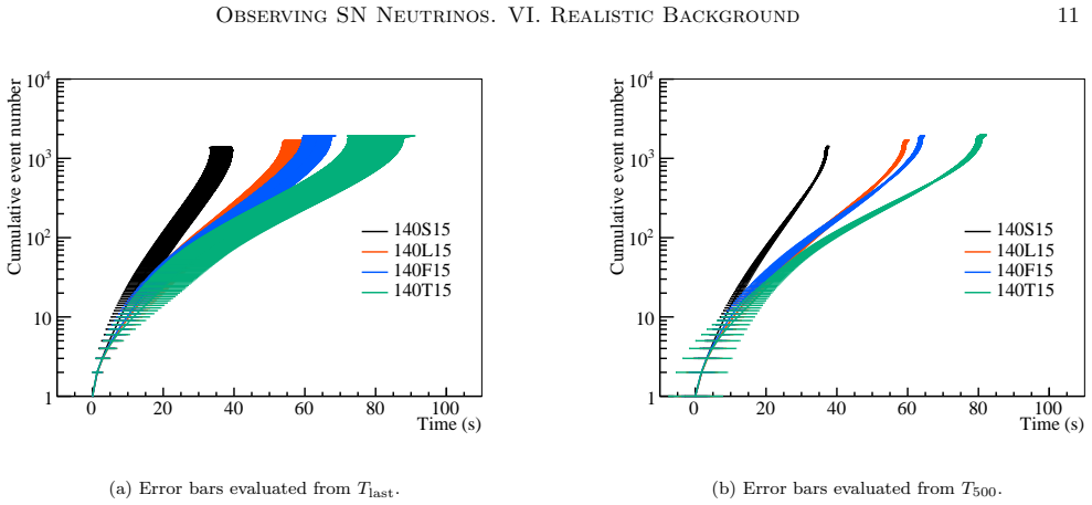
The paper's central discovery is that $T_{\rm last}$, the time of the last observed neutrino event selected with a 5-second sliding window and an 8 MeV energy threshold, carries enough information to differentiate between core-collapse supernova models with different proto-neutron-star masses and different nuclear equations of state. In particular, the Shen equation of state gives the shortest $T_{\rm last}$ and the Togashi equation of state the longest, with the LS220 and Furusawa-Togashi cases in between; the backward-time cumulative distribution from $T_{\rm last}$ and the time difference between the 500th-to-last and 1000th-to-last events sharpen the separation. A Bayesian calculation using these timing observables can constrain the equation of state, with shorter $T_{\rm last}$ indicating a lower central density and larger neutron-star radius, and longer $T_{\rm last}$ indicating abundant heavy nuclei near the surface.
Load-bearing premise
The load-bearing premise is that the background rate above 5 MeV in the fiducial volume after the spallation cut, $8.2\times10^{-3}\,\mathrm{s}^{-1}$ taken from Mori et al. (2022), is a known constant when choosing the 5 s / 8 MeV selection; if the real background rate or spectrum differs during a supernova burst, the $5\sigma$ thresholds and all $T_{\rm last}$ distributions shift.
Editorial extensions
If this is right
- A galactic supernova at 10 kpc could yield a measured $T_{\rm last}$ that separates the Shen and Togashi equations of state, with shorter $T_{\rm last}$ implying a less compact neutron star and longer $T_{\rm last}$ implying heavy nuclei near the surface.
- The backward-time cumulative distribution anchored at $T_{\rm last}$, and especially the time gap between the 500th-to-last and 1000th-to-last events, reduces statistical scatter and helps separate models with similar light curves such as LS220 and Furusawa-Togashi.
- Late-phase neutrino emission depends mainly on proto-neutron-star mass and radius, not on the progenitor's zero-age main-sequence mass; changing $M_{\rm ZAMS}$ from 15 to 40 solar masses leaves the late-phase timing information essentially unchanged.
- The same $T_{\rm last}$-based analysis can be applied to any neutrino detector with event-by-event timing, not only Super-Kamiokande.
Reading between the lines
- The authors do not draw this conclusion, but the $T_{\rm last}$ sliding window is a one-number summary of the event-time series; using the full spectrum of inter-event intervals on the same mock data could sharpen EOS discrimination further than the $T_{500}$--$T_{1000}$ gap alone.
- A testable extension is to apply the same background-aware framework to pre-supernova neutrinos from the silicon-burning phase, where the shorter emission window makes background treatment even more critical for an early-warning trigger.
- Scaling the same simulation to a larger water Cherenkov detector with a bigger fiducial volume should push the distance at which EOS separation works beyond 10 kpc, because the signal scales with detector mass while the background rate per kiloton stays roughly constant.
Signed reviews
Editorial analysis
A structured set of objections, weighed in public.
Referee Report
Summary. This paper develops a practical analysis framework for identifying the last supernova-neutrino event, Tlast, in Super-Kamiokande, with realistic backgrounds. Signal events are generated with SKSNSim for proto-neutron-star cooling models using four nuclear equations of state (Shen, LS220, Togashi, and Furusawa-Togashi) and several baryon masses, while background events are sampled from the in-situ SK measurement of Mori et al. (2022). After applying fiducial-volume and spallation cuts, the authors choose a time window Twid = 5 s and energy threshold Eth = 8 MeV, claim that these provide 5-sigma background rejection, and define Tlast as the last event found by a forward-sliding window. Tlast distributions from 1000 realizations are compared across models, and a backward-time analysis using the cumulative event count from Tlast and the time difference T500 - T1000 is used in a Bayesian model-selection calculation. The paper concludes that Tlast can differentiate core-collapse supernova models with different PNS masses and equations of state, and in particular that the Shen and Togashi EOSs can be effectively distinguished.
Significance. If the background-rejection step is quantitatively sound, this paper delivers a practical, ready-to-use recipe for the next galactic supernova and demonstrates that timing information alone carries EOS-discriminating power beyond the total event count. The strengths are the clearly specified Monte Carlo pipeline, the use of actual SK background rates from Mori et al. (2022), the large number of realizations, and the public release of the simulation code and neutrino light-curve data. The central new claim, however, rests on the unsupported assertion that background contamination is negligible, so the practical applicability claimed in the title and conclusion is not yet established.
major comments (3)
- [Section 3.3, Table 1] The 5-sigma background-rejection claim is not demonstrated by a transparent calculation. Section 3.2 gives the post-cut background rate as 8.2e-3 s^-1 above 5 MeV, and Section 3.3 states that Eth = 8 MeV rejects about 98% of background, yielding roughly 1.6e-4 s^-1 above 8 MeV. For the chosen Twid = 5 s, the expected number of background events per window is then about 8e-4, so the probability of observing at least one background event is about 8e-4, which is a roughly 3-sigma one-sided fluctuation rather than 5 sigma. The caption of Table 1 says all listed (Twid, Eth) pairs exclude background at greater than 5 sigma, but the Poisson calculation is not shown. Please provide the exact test, including whether it is one- or two-sided, which background rate is used, and how the Eth-dependent spectrum is integrated, and correct the criterion if the calculation does not reach 5 sigma.
- [Section 4.2, Figures 13 and 14] The assertion that the background impact in Figures 13 and 14 is negligible is unsupported because the promised comparison with background-free mock samples is not shown. The sliding-window algorithm searches the entire post-burst interval, so a lone background event after the true signal tail can define Tlast. With a background rate of approximately 1.6e-4 s^-1 above 8 MeV over a 200 s search, the expected number of such events is about 0.03, meaning a few percent of realizations will have a background event selected as Tlast. This biases Tlast late and preferentially affects the long-Tlast Togashi models that are central to the paper's discrimination claim. Please quantify the false-positive rate directly, report the with- and without-background Tlast distributions (for example by overlaying them), and revise the claim accordingly.
- [Section 3.2 and Section 3.3, Figure 3] The background rate and spectral shape are treated as fixed inputs with no uncertainty, yet they determine both the 5-sigma thresholds of Table 1 and all Tlast distributions. Since the background rate of 8.2e-3 s^-1 above 5 MeV is an empirical estimate, the robustness of the chosen Twid and Eth and of the final model-separation probabilities to plausible variations in this rate (for example a factor of two, or a different spectral index above 8 MeV) should be shown. Without such a sensitivity study, the claim that the analysis is realistic is not fully supported.
minor comments (5)
- [Section 5] In the conclusion, the symbol TSlast appears to be a typo for Tlast; please correct it.
- [Figures 13 and 14] The model labels in these figures are rendered as unreadable glyph sequences; please replace them with legible labels or a separate legend.
- [Section 3.3] The statement that Tlast is inconsistent with the measured background at more than 5 sigma significance should specify whether the significance is one-sided or two-sided and how the sliding-window search over time is treated.
- [Section 4.2, Equation (4)] The Bayesian probabilities are computed with PDFs obtained from the same simulation pipeline that generated the mock data; a sentence stating that the quoted percentages are an in-sample, idealized upper bound on discrimination would prevent over-interpretation.
- [Section 1] The first paragraph contains a stray phrase, 'and makes their observation', after a citation; please fix the grammar.
Circularity Check
No circularity found: the Tlast analysis is a forward-model sensitivity study; the claimed model discrimination follows from simulated signal properties, not from fitting or self-citation.
full rationale
The paper’s derivation chain is a forward simulation: PNS cooling models from the publicly released Paper I/II simulations are input to SKSNSim to generate signal events; backgrounds are drawn from the measured SK rate of Mori et al. (2022); Tlast is defined by a sliding-window algorithm whose (Twid, Eth) are chosen solely from the background rate under Poisson statistics; and the Tlast PDFs and Bayesian posteriors are computed from the same simulated samples. No parameter is fitted to the claimed outcome, and no uniqueness theorem or prior result by the authors is invoked to forbid alternatives. The fact that the Bayesian PDFs are generated from the same models used to produce mock observations makes this an in-sample sensitivity study, not a circular derivation: the EOS separation visible in Tlast is a property of the forward-modeled signal, not an input assumption. Self-citations to Papers I/II supply input physics and methods, but the central claim is derived by simulation rather than assumed from those citations. The skeptic’s concern about the unquantified 5-sigma background/trials correction is a statistical robustness issue, not a circularity, and does not affect this verdict.
Assumptions & free parameters
free parameters (6)
- Analysis time window Twid =
5 s
- Energy threshold Eth =
8.0 MeV
- 5-sigma detection significance requirement =
5 sigma (Poisson)
- Supernova distance D =
10 kpc
- Spallation cut signal loss =
20%
- Uniform model prior =
1/32 per model
assumptions (5)
- domain assumption PNS cooling light curves from Papers I/II (flux-limited diffusion, spherical symmetry) faithfully represent late-phase neutrino emission.
- domain assumption The SK background rate above 5 MeV after FV and spallation cuts (8.2e-3 s^-1) from Mori et al. (2022) is constant during a supernova burst.
- domain assumption Initial conditions for Furusawa-Togashi models are identical to Togashi models because early PNS matter is uniform.
- standard math Strumia-Vissani IBD cross section and SKSNSim detector response are accurate for sub-100 MeV neutrinos.
- standard math Event counts follow Poisson statistics for background rejection.
Cite this review
Pith. "Pith review of Observing Supernova Neutrino Light Curves with Super-Kamiokande.VI. A Practical Data Analysis Technique Considering Realistic Experimental Backgrounds." pith.science (2026). https://pith.science/paper/NUK5T5H4
@misc{pith2026250519721,
  author       = {Pith},
  title        = {Pith review of: Observing Supernova Neutrino Light Curves with Super-Kamiokande.VI. A Practical Data Analysis Technique Considering Realistic Experimental Backgrounds},
  year         = {2026},
  howpublished = {\url{https://pith.science/paper/NUK5T5H4}},
  note         = {Machine review of arXiv:2505.19721}
}
read the original abstract
Neutrinos from supernovae, especially those emitted during the late phase of core collapse, are essential for understanding the final stages of massive star evolution. We have been dedicated to developing methods for the analysis of neutrinos emitted during the late phase and observed at Super-Kamiokande (SK). Our previous studies have successfully demonstrated the potential of various analysis methods in extracting essential physical properties; however, the lack of background consideration has limited their practical application. In this study, we address this issue by incorporating a realistic treatment of the experimental signal and background events with the on-going SK experiment. We therefore optimize our analysis framework to reflect realistic observational conditions, including both signal and background events. Using this framework we study several long-time supernova models, simulating the late phase neutrino observation in SK and focusing in particular on the identification of the last observed event. We discuss the possibility of model discrimination methods using timing information from this last observed event.
Figures


Figures from the paper (11 more)




Reference graph
Works this paper leans on
-
[1]
2018, arXiv e-prints, arXiv:1805.04163, doi: 10.48550/arXiv.1805.04163
Abe, K., Abe, K., Aihara, H., et al. 2018, arXiv e-prints, arXiv:1805.04163, doi: 10.48550/arXiv.1805.04163
-
[2]
2024, PhRvD, 109, 092001, doi: 10.1103/PhysRevD.109.092001
Abe, K., Bronner, C., Hayato, Y., et al. 2024, PhRvD, 109, 092001, doi: 10.1103/PhysRevD.109.092001
-
[3]
2022, ApJ, 934, 85, doi: 10.3847/1538-4357/ac7a3f
Abe, S., Asami, S., Eizuka, M., et al. 2022, ApJ, 934, 85, doi: 10.3847/1538-4357/ac7a3f
-
[4]
Abi, B., Acciarri, R., Acero, M. A., et al. 2020, JINST, 15, T08008, doi: 10.1088/1748-0221/15/08/T08008
-
[5]
2023, ApJ, 944, 60, doi: 10.3847/1538-4357/acad76
Akaho, R., Harada, A., Nagakura, H., et al. 2023, ApJ, 944, 60, doi: 10.3847/1538-4357/acad76
-
[6]
Volchenko, V. I. 1988, Phys. Lett. B, 205, 209, doi: 10.1016/0370-2693(88)91651-6
-
[7]
An, F., An, G., An, Q., et al. 2016, J. Phys. G, 43, 030401, doi: 10.1088/0954-3899/43/3/030401
-
[8]
Bionta, R. M., Blewitt, G., Bratton, C. B., et al. 1987, PhRvL, 58, 1494, doi: 10.1103/PhysRevLett.58.1494
Show all 49 references
-
[9]
M., Mazurek, T
Burrows, A., Lattimer, J. M., Mazurek, T. J., & Yahil, A. 1987, Research in astrophysics: Stellar collapse and supernovae, Termination Report, 1 Aug. 1980 - 30 Nov. 1986 State Univ. of New York, Stony Brook
1987
-
[10]
2003, Nucl
Fukuda, S., Fukuda, Y., Hayakawa, T., et al. 2003, Nucl. Instrum. Methods Phys. Res. A, 501, 418, doi: 10.1016/S0168-9002(03)00425-X
2003 doi
-
[11]
Furusawa, S., Togashi, H., Nagakura, H., et al. 2017, J. Phys. G, 44, 094001, doi: 10.1088/1361-6471/aa7f35
2017 doi
-
[12]
Harada, A. 2023, SPECIAL BLEND: Supernova Parameter Estimation Code based on Insight on Analytic Late-time Burst Light curve at Earth Neutrino Detector, 1.0, Zenodo, doi: 10.5281/zenodo.8004041
2023 doi
-
[13]
2023, ApJ, 954, 52, doi: 10.3847/1538-4357/ace52e
Harada, A., Suwa, Y., Harada, M., et al. 2023, ApJ, 954, 52, doi: 10.3847/1538-4357/ace52e
2023 doi
-
[14]
1987, PhRvL, 58, 1490, doi: 10.1103/PhysRevLett.58.1490
Hirata, K., Kajita, T., Koshiba, M., et al. 1987, PhRvL, 58, 1490, doi: 10.1103/PhysRevLett.58.1490
1987 doi
-
[15]
Horiuchi, S., & Kneller, J. P. 2018, J. phys. G, 45, 043002, doi: 10.1088/1361-6471/aaa90a
2018 doi
-
[16]
2017, in Handbook of Supernovae, ed
Janka, H.-T. 2017, in Handbook of Supernovae, ed. A. W. Alsabti & P. Murdin, 1575, doi: 10.1007/978-3-319-21846-5 4
2017 doi
-
[17]
2024, ApJ, 970, 93, doi: 10.3847/1538-4357/ad4d8e
Kashiwagi, Y., Abe, K., Bronner, C., et al. 2024, ApJ, 970, 93, doi: 10.3847/1538-4357/ad4d8e
2024 doi
-
[18]
2020, Annu
Kato, C., Ishidoshiro, K., & Yoshida, T. 2020, Annu. Rev. Nucl. Part. Sci., 70, 121, doi: 10.1146/annurev-nucl-040620-021320
2020 doi
-
[19]
2006, Rep
Kotake, K., Sato, K., & Takahashi, K. 2006, Rep. Prog. Phys., 69, 971, doi: 10.1088/0034-4885/69/4/R03
2006 doi
-
[20]
M., & Swesty, D
Lattimer, J. M., & Swesty, D. F. 1991, Nucl. Phys. A, 535, 331, doi: https://doi.org/10.1016/0375-9474(91)90452-C
1991 doi
- [21]
-
[22]
W., Roberts, L
Li, S. W., Roberts, L. F., & Beacom, J. F. 2021, PhRvD, 103, 023016, doi: 10.1103/PhysRevD.103.023016
2021 doi
-
[23]
2024, PhRvD, 110, 032003, doi: 10.1103/PhysRevD.110.032003
Locke, S., Coffani, A., Abe, K., et al. 2024, PhRvD, 110, 032003, doi: 10.1103/PhysRevD.110.032003
2024 doi
-
[24]
2021, Prog
Mori, M., Suwa, Y., Nakazato, K., et al. 2021, Prog. Theor. Exp. Phys., 2021, 023E01, doi: 10.1093/ptep/ptaa185
2021 doi
-
[25]
2022, ApJ, 938, 35, doi: 10.3847/1538-4357/ac8f41
Mori, M., Abe, K., Hayato, Y., et al. 2022, ApJ, 938, 35, doi: 10.3847/1538-4357/ac8f41
2022 doi
-
[26]
2021, MNRAS, 500, 696, doi: 10.1093/mnras/staa2691
Nagakura, H., Burrows, A., Vartanyan, D., & Radice, D. 2021, MNRAS, 500, 696, doi: 10.1093/mnras/staa2691
2021 doi
-
[27]
2025, SKSNSim: Supernova burst and Diffuse Supernova Neutrino Background simulator for Water Cherenkov Detectors, 1.2.3a, Zenodo, doi: 10.5281/zenodo.16751274
Nakanishi, F. 2025, SKSNSim: Supernova burst and Diffuse Supernova Neutrino Background simulator for Water Cherenkov Detectors, 1.2.3a, Zenodo, doi: 10.5281/zenodo.16751274
2025 doi
-
[28]
2024, ApJ, 965, 91, doi: 10.3847/1538-4357/ad344e
Nakanishi, F., Izumiyama, S., Harada, M., & Koshio, Y. 2024, ApJ, 965, 91, doi: 10.3847/1538-4357/ad344e
2024 doi
-
[29]
2022, Supernova Neutrino Light Curves from Proto-Neutron Star Cooling with Various Nuclear Equation of State, 1.0, Zenodo, doi: 10.5281/zenodo.5778223
Nakazato, K. 2022, Supernova Neutrino Light Curves from Proto-Neutron Star Cooling with Various Nuclear Equation of State, 1.0, Zenodo, doi: 10.5281/zenodo.5778223
2022 doi
-
[30]
2013, ApJS, 205, 2, doi: 10.1088/0067-0049/205/1/2
Nakazato, K., Sumiyoshi, K., Suzuki, H., et al. 2013, ApJS, 205, 2, doi: 10.1088/0067-0049/205/1/2
2013 doi
-
[31]
2019, ApJ, 878, 25, doi: 10.3847/1538-4357/ab1d4b —
Nakazato, K., & Suzuki, H. 2019, ApJ, 878, 25, doi: 10.3847/1538-4357/ab1d4b —. 2020, ApJ, 891, 156, doi: 10.3847/1538-4357/ab7456
2019 doi
-
[32]
2018, PhRvC, 97, doi: 10.1103/physrevc.97.035804
Nakazato, K., Suzuki, H., & Togashi, H. 2018, PhRvC, 97, doi: 10.1103/physrevc.97.035804
2018 doi
-
[33]
2022, ApJ, 925, 98, doi: 10.3847/1538-4357/ac3ae2 O’Connor, E., & Ott, C
Nakazato, K., Nakanishi, F., Harada, M., et al. 2022, ApJ, 925, 98, doi: 10.3847/1538-4357/ac3ae2 O’Connor, E., & Ott, C. D. 2013, ApJ, 762, 126, doi: 10.1088/0004-637X/762/2/126
2022 doi
-
[34]
1987, Phys
Sato, K., & Suzuki, H. 1987, Phys. Lett. B, 196, 267, doi: 10.1016/0370-2693(87)90728-3
1987 doi
-
[35]
2012, Annu
Scholberg, K. 2012, Annu. Rev. Nucl. Part. Sci., 62, 81, doi: 10.1146/annurev-nucl-102711-095006
2012 doi
-
[36]
1998, Nucl
Shen, H., Toki, H., Oyamatsu, K., & Sumiyoshi, K. 1998, Nucl. Phys. A, 637, 435, doi: https://doi.org/10.1016/S0375-9474(98)00236-X —. 2011, ApJS, 197, 20, doi: 10.1088/0067-0049/197/2/20
1998 doi
-
[37]
2003, Phys
Strumia, A., & Vissani, F. 2003, Phys. Lett. B, 564, 42, doi: 10.1016/s0370-2693(03)00616-6
2003 doi
-
[38]
2023, Prog
Sumiyoshi, K., Furusawa, S., Nagakura, H., et al. 2023, Prog. Theor. Exp. Phys., 2023, 013E02, doi: 10.1093/ptep/ptac167
2023 doi
-
[39]
2005, ApJ, 629, 922, doi: 10.1086/431788
Sumiyoshi, K., Yamada, S., Suzuki, H., et al. 2005, ApJ, 629, 922, doi: 10.1086/431788
2005 doi
-
[40]
2014, PASJ, 66, L1, doi: 10.1093/pasj/pst030 16 Nakanishi et al
Suwa, Y. 2014, PASJ, 66, L1, doi: 10.1093/pasj/pst030 16 Nakanishi et al
2014 doi
-
[41]
2019, ApJ, 881, 139, doi: 10.3847/1538-4357/ab2e05
Suwa, Y., Sumiyoshi, K., Nakazato, K., et al. 2019, ApJ, 881, 139, doi: 10.3847/1538-4357/ab2e05
2019 doi
-
[42]
2022, ApJ, 934, 15, doi: 10.3847/1538-4357/ac795e
Suwa, Y., Harada, A., Harada, M., et al. 2022, ApJ, 934, 15, doi: 10.3847/1538-4357/ac795e
2022 doi
-
[43]
2025, ApJ, 980, 117, doi: 10.3847/1538-4357/adabe2
Suwa, Y., Harada, A., Mori, M., et al. 2025, ApJ, 980, 117, doi: 10.3847/1538-4357/adabe2
2025 doi
-
[44]
1994, in Physics and Astrophysics of Neutrinos, XIII, ed
Suzuki, H. 1994, in Physics and Astrophysics of Neutrinos, XIII, ed. M. Fukugita & A. Suzuki, 420
1994
-
[45]
2018, MNRAS, 475, L91, doi: 10.1093/mnrasl/sly008
Takiwaki, T., & Kotake, K. 2018, MNRAS, 475, L91, doi: 10.1093/mnrasl/sly008
2018 doi
-
[46]
A., Burrows, A., & Pinto, P
Thompson, T. A., Burrows, A., & Pinto, P. A. 2003, ApJ, 592, 434, doi: 10.1086/375701
2003 doi
-
[47]
2017, NuPhA, 961, 78, doi: 10.1016/j.nuclphysa.2017.02.010
Togashi, H., Nakazato, K., Takehara, Y., et al. 2017, NuPhA, 961, 78, doi: 10.1016/j.nuclphysa.2017.02.010
2017 doi
-
[48]
2013, NuPhA, 902, 53, doi: 10.1016/j.nuclphysa.2013.02.014
Togashi, H., & Takano, M. 2013, NuPhA, 902, 53, doi: 10.1016/j.nuclphysa.2013.02.014
2013 doi
- [49]
Reviewed August 7, 2026 · model on record in the stance chip above.
Discussion (0). Continue with ORCID to comment.