REVIEW 4 major objections 5 minor 1 cited by
Rectified LpJEPA: Joint-Embedding Predictive Architectures with Sparse and Maximum-Entropy Representations
T0 review · 4 major / 5 minor · reviewed 2026-08-03 · deepseek-v4-flash
Pith's one-line read Rectified LpJEPA matches JEPA representations to a Rectified Generalized Gaussian target, giving users direct control over the expected fraction of zero entries while preserving maximum-entropy structure and, empirically, downstream accurac
desk verdict Useful regularizer with careful math, but the headline sparsity-tracking claim rests on single-seed runs and a few loose ends; deserves a thorough referee. read the letter →
The pith
A machine-rendered reading of the paper's core claim, the machinery that carries it, and where it could break.
The reading
What carries the argument
Rectified Distribution Matching Regularization (RDMReg): a sliced two-sample loss, instantiated as sliced 2-Wasserstein distance, that matches one-dimensional projections of rectified features to projections of samples from a Rectified Generalized Gaussian (RGG) distribution. RGG is a mixture of a point mass at zero and a truncated generalized Gaussian on (0,∞), with parameters (µ, σ, p); its expected ℓ0 norm is d·Φ(µ/σ), so the target's sparsity is chosen in advance. Because RGG is not closed under linear projections, the Cramér–Wold device cannot reduce the match to a parametric family per projection, which is why the loss is nonparametric and two-sample.
What would settle it
Train Rectified LpJEPA at µ=−3, p=2 on a standard benchmark across several seeds and measure per-coordinate variance and the fraction of nonzero entries: if the empirical ℓ0 norm departs systematically from d·Φ(µ/σ), or if the representation collapses (variance→0) while the RDMReg loss is near zero, the sparsity-transfer claim fails.
Extended reading notes
Core claim
Central claim: sparsity and non-negativity can be imposed on JEPA representations by changing the target distribution rather than adding explicit ℓ0 or ℓ1 penalties. The paper introduces the Rectified Generalized Gaussian (RGG)—a Dirac mass at zero mixed with a truncated generalized Gaussian on the positive reals—and proves it is maximum-entropy under an expected ℓp-norm constraint on the positive orthant. Rectified LpJEPA matches projected feature marginals to RGG samples through sliced two-sample distribution matching (RDMReg). The paper argues this strictly generalizes Gaussian-based JEPA regularization and reports that learned features track the target's expected ℓ0 norm, with accuracy d
Load-bearing premise
The empirical claim that features track the target's expected ℓ0 norm at extreme sparsity assumes the RDMReg term continues to dominate the invariance term even when the target's per-coordinate variance is tiny (about 0.0002 at µ=−3), a regime where no theorem guarantees non-collapsed optima.
Editorial extensions
If this is right
- Sparsity becomes a selectable property: choosing (µ, σ, p) for the target RGG sets the expected fraction of nonzero output entries, and the learned features track that fraction across backbones.
- Gaussian-based JEPA regularization is recovered as the dense edge case (p=2, no rectification), so the method is a strict generalization rather than an alternative.
- Sparse, non-negative features can be obtained without negative pairs, reconstruction, or explicit ℓ0 penalties, retaining competitive linear-probe accuracy until roughly 95% of entries are zero.
- Matching to RGG implicitly drives the feature covariance toward a scaled identity, so second-order collapse is controlled with a linear number of projections.
- Representation sparsity varies systematically across downstream datasets after one pretraining, providing a potential signal for out-of-distribution detection.
Reading between the lines
- Because the RGG family is not closed under linear projections, the method's reliance on nonparametric two-sample matching suggests that other sliced divergences (e.g., energy-based or kernel-based) could substitute for the sliced 2-Wasserstein loss; the paper's theory does not single out one metric.
- The maximum-entropy derivation extends beyond the exponential family: any truncated exponential-family density on the positive reals mixed with a Dirac mass at zero would give controllable ℓ0 sparsity with an analogous entropy guarantee, so the rectified generalized Gaussian is one member of a broader design space.
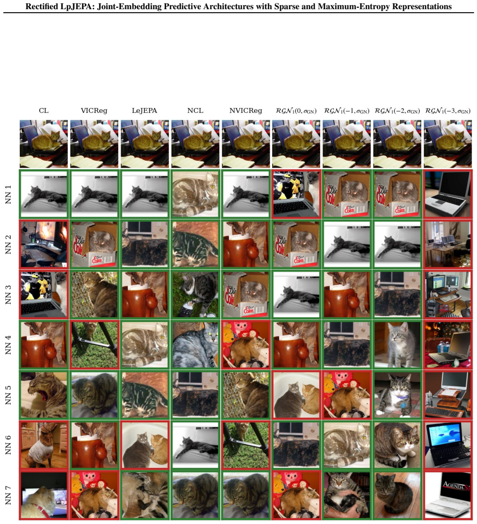
- At extreme sparsity the paper's own qualitative analysis shows retrieval flips between competing scene factors rather than losing information; a testable consequence is that sparsity acts as a feature-selection prior, and combining it with explicit decorrelation at tiny µ might preserve accuracy further.
- The fixed-σGN choice makes target per-coordinate variance shrink sharply as µ becomes very negative; an editor's reading is that a variance-normalized target or a feature-whitening step could push the Pareto frontier past roughly 95% sparsity, but the paper does not claim this.
Editorial analysis
A structured set of objections, weighed in public.
Referee Report
Summary. The paper introduces Rectified LpJEPA, a JEPA variant whose features are passed through ReLU and regularized by RDMReg, a sliced two-sample distribution-matching loss that aligns the feature distribution to a Rectified Generalized Gaussian (RGG) target. The RGG family is a mixture of a Dirac at zero and a truncated Generalized Gaussian, parameterized by (μ, σ, p). The authors derive closed-form moments, an expected ℓ0 formula, maximum-entropy characterizations for the truncated family, and a Rényi information-dimension characterization for the rectified family. They argue that RDMReg strictly generalizes LeJEPA, induces controllable sparsity, preserves task-relevant information, and achieves favorable sparsity–performance trade-offs. Empirical results on CIFAR-100 and ImageNet-100 compare Rectified LpJEPA against dense and sparse baselines using linear probing and transfer evaluations.
Significance. If the main claims hold, the paper makes a useful contribution to distribution-based collapse prevention in JEPAs by adding a principled sparsity and non-negativity axis to the existing Gaussian-matching framework. The theoretical appendices are a clear strength: Proposition B.9 gives closed-form moments, Proposition 3.3 gives a maximum-entropy derivation for truncated Generalized Gaussians, and Theorem 3.6 gives a careful Rényi information-dimension treatment of the rectified family. The claim that Rectified LpJEPA strictly generalizes LeJEPA is credible. The significance is currently limited by the empirical support: the central sparsity-transfer claim rests on single-seed runs, a partially circular figure, and a large discrepancy at extreme sparsity. With multi-seed results, error bars, and a sharper analysis of the high-sparsity regime, the paper would be a solid contribution.
major comments (4)
- [§5.4, Fig. 3b, Table 1] The central 'controllable sparsity' claim is not established at high sparsity. The only direct evidence is Fig. 3b, which has no error bars and plots the empirical ℓ0 against the target value from Proposition 3.5. Because the training objective (Eq. 16) matches the feature distribution to the RGG target, this agreement is a check that the regularizer worked, not an independent prediction. More concretely, Table 1 reports RGN2(−2.5, σGN) with normalized ℓ0 = 0.0224, whereas Proposition 3.5 gives Φ(μ/σ) ≈ 0.0062, a 3.6× discrepancy. The visual closeness in Fig. 3b therefore overstates agreement at extreme sparsity. Please report per-seed error bars, a quantitative mismatch curve, and an analysis of dependence on batch size and number of projections.
- [§4.5, Eqs. (14)–(16), Fig. 6d] There is no argument that the joint objective has non-degenerate optima with the target sparsity. For RGN2(−3, σGN), the per-coordinate variance after rectification is about 2×10⁻⁴ (Fig. 6d), while the RDMReg term uses B=128 samples and N=8192 projections and is not an ℓ0 penalty. In this regime, the sliced 2-Wasserstein gradient can be small relative to the invariance term, and because the features use plain ReLU, high measured sparsity could reflect dead units rather than controlled matching of the RGG tail. Section 4.5 only asserts 'σ > ε ... to prevent collapse'; no theorem or diagnostic supports non-collapse. Please add a collapse/dead-unit analysis (effective rank, dead-unit fraction, gradient norms of the two loss terms) and a batch-size/projection sweep in the high-sparsity regime.
- [§5.8, Table 1, Appendix L.8] All ImageNet-100 pretraining results are reported from a single run (seed 5). The headline comparisons show small gaps — e.g., RGN2(0, σGN) encoder accuracy 85.08 vs. LeJEPA 84.80 and VICReg 84.18 — and no variance or significance is reported. This is insufficient support for the abstract's and Section 6's claims of 'favorable sparsity–performance trade-offs' and 'competitive downstream performance.' Please report means and standard deviations over at least 3–5 seeds for the main configurations, and state whether the differences are significant.
- [§3.5, Theorem 3.6] The wording in Section 3.5 — 'rectifications still preserve the maximal entropy property ... up to rescaling' — is not supported by a variational statement. Proposition 3.3 maximizes differential entropy over continuous densities on a support S under an E∥x∥_p^p constraint. Theorem 3.6 only computes the Rényi information dimension and d(ξ)-dimensional entropy of the RGG family; it does not prove that RGG maximizes any entropy among distributions with a given expected ℓ0 or a given Dirac-mixing probability. To make the claimed maximum-entropy property precise, the authors should either state and prove a maximization result over a well-defined class of mixtures, or temper the language.
minor comments (5)
- [§4.2, Appendix L.5] The objective is written without weights in Eqs. (14)–(15), but Appendix L.5 reports λ_sim = 25.0 and λ_dist = 125.0. The exact weighted objective should appear in the main text for reproducibility.
- [Fig. 3a, §5.2] The notation 'z+', 'p z+', and 'p z' in the figure and text is not defined before use. Please define z+ := ReLU(z) and the target-distribution shorthand in the caption or in Section 4.
- [Algorithm 2] The bisection search assumes initial bounds σ_L and σ_U with f(σ_L) < 0 and f(σ_U) > 0, but the existence and construction of such bounds are not discussed. A brief justification or a practical initialization would help.
- [Appendix D.1] There is a typo: 'Genealized' should be 'Generalized' in the section heading.
- [§5.4, Fig. 3b] The figure legend says results span ResNet, ViT, and ConvNeXt, but no per-backbone error bars or per-backbone breakdown is shown. It would be clearer to plot each backbone separately or report across-backbone variance.
Circularity Check
Sparsity tracking in Fig. 3b is a self-consistency check: the 'theoretical ℓ0 prediction' is the ℓ0 of the same RGG distribution used as the RDMReg target, so the agreement is built into the objective rather than an independent prediction.
-
self definitional
[Section 5.4, Figure 3b; Proposition 3.5 / Eq. (9) vs. RDMReg Eq. (16)]
"In Figure 3b, we show both the empirical ℓ0 norms measured over different pretrained backbones ... and the theoretical ℓ0 norm computed using Equation (9) ... We observe that across different mean shift values µ on the x-axis, the empirical ℓ0 closely tracks the theoretical predictions."
The 'theoretical prediction' Eq. (9) is the expected ℓ0 of the target distribution RGN_p(μ,σ) from Proposition 3.5. RDMReg (Eq. 16) explicitly matches feature projections to samples y∼RGN_p(μ,σ) drawn from that same distribution. Therefore the empirical ℓ0 tracking reported in Fig. 3b is a consistency check that the distribution-matching regularizer drove the features toward the chosen target; it is not an independent prediction of sparsity from first principles. The headline capability 'controllable sparsity' is a design property of the target distribution inserted into the loss, so the Fig. 3b agreement reduces, by construction, to the success of the matching objective rather than to a separate theoretical consequence.
full rationale
The core mathematical propositions (Prop. 3.3 max entropy under ℓp constraints; Prop. 3.5 expected ℓ0 of RGN_p) are standard or direct calculus and are not circular: they derive properties of distributions, and the paper does not fit parameters to the data used to evaluate those properties. The main circularity concern is located in the empirical validation of 'controllable sparsity' (Section 5.4, Fig. 3b). Because RDMReg is defined as a sliced Wasserstein match between feature projections and samples from RGN_p(μ,σ), and Prop. 3.5 computes the ℓ0 of exactly that RGN_p(μ,σ), the plotted 'theoretical prediction' is a property of the loss's own target. The empirical tracking then primarily verifies that the regularizer converged, rather than providing independent support for a sparsity law. This is a partial circularity of the validation framing, but it does not invalidate the method's empirical benchmark comparisons (Tables 1-8), which are externally evaluated. The paper's self-citations (e.g., LeJEPA, Radial-VCReg) are not load-bearing for the derivation: they are precedents and baselines, and the central dependence is on classical entropy results and the Cramér-Wold device. Claims that RGG 'preserves maximum-entropy up to rescaling' under sparsity constraints go beyond what is proved (Theorem 3.6 computes an entropy but does not prove maximality among mixtures with the same ℓ0), but this is an overclaim rather than a circular reduction. Overall, the derivation is not wholly circular, but one headline 'prediction' is self-referential, warranting a moderate score.
Assumptions & free parameters
free parameters (5)
- Target mean shift µ =
swept in {-3,...,1}
- Target shape p =
0.25, 0.5, 0.75, 1.0, 2.0
- Target scale σ =
σ_GN (default) or σ_RGN via bisection
- Loss weights λ_sim, λ_dist =
25.0, 125.0 (Appendix L.5)
- Number of projections N =
8192
assumptions (6)
- standard math Maximum-entropy variational characterization (Lemma E.1): max-entropy density subject to moment constraints has exponential form.
- standard math Cramér–Wold device: equality of all 1D projected distributions implies equality of multivariate distributions.
- standard math Rényi information dimension decomposition for mixed discrete/continuous measures (Definition F.3).
- domain assumption For p∈{1,2}, zero-mean generalized Gaussian admits radial-angular decomposition with uniform angular distribution (Barthe et al. 2005; Alonso-Gutierrez et al. 2018).
- ad hoc to paper Finite-projection sliced 2-Wasserstein distance is a faithful surrogate for full distribution matching in the training objective.
- domain assumption Anti-collapse: the distribution-matching term dominates the invariance term even when the target variance is very small.
invented entities (1)
-
Rectified Generalized Gaussian (RGG) distribution family
Cite this review
Pith. "Pith review of Rectified LpJEPA: Joint-Embedding Predictive Architectures with Sparse and Maximum-Entropy Representations." pith.science (2026). https://pith.science/paper/QN73CTOV
@misc{pith2026260201456,
  author       = {Pith},
  title        = {Pith review of: Rectified LpJEPA: Joint-Embedding Predictive Architectures with Sparse and Maximum-Entropy Representations},
  year         = {2026},
  howpublished = {\url{https://pith.science/paper/QN73CTOV}},
  note         = {Machine review of arXiv:2602.01456}
}
abstract
Joint-Embedding Predictive Architectures (JEPA) learn view-invariant representations and admit projection-based distribution matching for collapse prevention. Existing approaches regularize representations towards isotropic Gaussian distributions, but inherently favor dense representations and fail to capture the key property of sparsity observed in efficient representations. We introduce Rectified Distribution Matching Regularization (RDMReg), a sliced two-sample distribution-matching loss that aligns representations to a Rectified Generalized Gaussian (RGG) distribution. RGG enables explicit control over expected $\ell_0$ norm through rectification, while its continuous truncated component admits a maximum-entropy characterization under expected $\ell_p$ norm and support constraints. Equipping JEPAs with RDMReg yields Rectified LpJEPA, which strictly generalizes prior Gaussian-based JEPAs. Empirically, Rectified LpJEPA learns sparse, non-negative representations with favorable sparsity--performance trade-offs and competitive downstream performance on image classification benchmarks, showing that RDMReg can enforce sparsity while preserving task-relevant information.
Figures


Figures from the paper (16 more)




Forward citations
Cited by 1 Pith paper
-
VISReg: Variance-Invariance-Sketching Regularization for JEPA training
VISReg replaces covariance in VICReg-style objectives with sliced-Wasserstein sketching for JEPA training, claiming better OOD performance and resilience to collapse.
Reference graph
Works this paper leans on
-
[1997]
cc/paper_files/paper/1997/file/ 28fc2782ea7ef51c1104ccf7b9bea13d-Paper
URL https://proceedings.neurips. cc/paper_files/paper/1997/file/ 28fc2782ea7ef51c1104ccf7b9bea13d-Paper. pdf. Subbotin, M. T. On the law of frequency of error.Mat. Sb., 31(2):296–301, 1923. MathNet, zbMATH. Tibshirani, R. Regression shrinkage and selection via the lasso.Journal of the Royal Statistical Society Series B: Statistical Methodology, 58(1):267–...
arXiv 1997
-
[2000]
cc/paper_files/paper/2000/file/ f9d1152547c0bde01830b7e8bd60024c-Paper
URL https://proceedings.neurips. cc/paper_files/paper/2000/file/ f9d1152547c0bde01830b7e8bd60024c-Paper. pdf. Lee, D. D. and Seung, H. S. Learning the parts of objects by non-negative matrix factorization.nature, 401(6755): 788–791, 1999. Lehmann, E. L. and Romano, J. P.Testing Statistical Hy- potheses. Wiley, 1951. Liu, Z., Mao, H., Wu, C.-Y ., Feichtenh...
arXiv 2000
-
[2025]
and LeJEPA (Balestriero & LeCun, 2025) go beyond second-order dependencies by learning isotropic Gaussian features. Our Rectified LpJEPA also reduce higher-order dependencies by design, while enforcing sparsity over learned representations. Prior work like Non-Negative Contrastive learning (NCL) (Wang et al., 2024) also aims to learn sparse features by op...
arXiv 2025
Reviewed August 3, 2026 · model on record in the stance chip above.
Discussion (0). Sign in to comment.