REVIEW 3 major objections 5 minor 6 references
The Cost of Learning Under Multiple Change Points
T0 review · 3 major / 5 minor · reviewed 2026-08-03 · deepseek-v4-flash
Pith's one-line read Near-minimax tracking of a changing mean is achievable without knowing the horizon or number of changes.
desk verdict Solid upper-bound analysis and a genuinely new SNR-degradation lemma, but Theorem 4.2's minimax claim is overstated because the lower bound silently assumes M ≥ cσ. read the letter →
The pith
A machine-rendered reading of the paper's core claim, the machinery that carries it, and where it could break.
The reading
What carries the argument
The central object is the ATC detection statistic, a CUSUM-style scan over split points whose threshold grows logarithmically with time since the last restart. The mechanism that carries the argument is the SNR-degradation bound: after a missed change, the loss in detection signal-to-noise ratio for the next change is bounded by the signal-to-noise ratio of the missed change itself (Lemma 3.1, with the two-change algebraic identity in Claim A.12). This caps the cascading 'endogenous confounding' effect at a logarithmic scale, which is what converts the bias term from a potential linear cost into O(σ²S log T).
What would settle it
Run ATC on a three-segment Gaussian environment with segment lengths (n0, n1, n2) = (1000, 10, 100) and means (0, 0.1, 1), so that the first change is just below the detection threshold and is missed; then measure the effective SNR for the second change over time. If the SNR loss (SNR⋆_2 − SNR^eff_2) ever exceeds the SNR of the missed first change evaluated at τ2, Lemma 3.1 is violated, and the O(σ²S log T) bound would not hold in that regime. A less algorithmic test: directly compute the two SNRs from the formulas in Claim A.12 with these parameters.
Extended reading notes
Core claim
The paper's central claim is that the minimax dynamic regret for online tracking of a piecewise-constant mean with S changes is Θ(σ²S log(T/S)) (up to lower-order terms), and that this rate is achievable by a specific anytime algorithm, ATC, that does not know T or S. The proof relies on a novel bound on the degradation of detection signal-to-noise ratio after missed detections: the loss in SNR for a change is at most the SNR of the most recently missed change. This quantization of the confounding effect leads to a logarithmic bias term and establishes that missed detections are analytically benign if the detector's threshold grows logarithmically. The lower bound formalizes the intuition th
Load-bearing premise
The proof depends on the inequality that after a missed change, the detection signal-to-noise ratio for the following change degrades by no more than the signal of the missed change itself; if that inequality fails in some multi-change path, the logarithmic regret guarantee breaks.
Editorial extensions
If this is right
- ATC achieves near-minimax regret without knowing the horizon T or the number of changes S, and without any detectability or spacing assumptions.
- The lower bound identifies the unavoidable cost of non-stationarity: each of the S changes contributes a logarithmic factor to the worst-case regret.
- Sublinear regret is achievable for any vanishing density of changes (S = o(T)); when S is proportional to T, regret becomes linear, as expected.
- The results imply that selective detection—deliberately missing small or brief shifts—is not just a heuristic but a principled strategy for online tracking.
- In practice, the algorithm's only required inputs are the noise proxy σ and an error budget α, making it a ready-to-use anytime method.
Reading between the lines
- The log(S) gap between the upper and lower bounds is likely closable by a horizon-aware algorithm that restarts on a fixed schedule of T/(S+1) rounds, as the authors conjecture; constructing such an algorithm and proving the matching O(σ²S log(T/S)) bound would tighten the result.
- The SNR-degradation principle may transfer to other sequential decision problems, such as bandits with switching or online compression, where a missed change contaminates a reference statistic; a testable extension is to check whether analogous logarithmic bounds hold under different losses (the paper notes L1 leads to Ω(√(ST))).
- The appendix's observation that an underestimated variance proxy σ causes false alarms to diverge suggests a practical research direction: designing an adaptive, data-driven σ calibration to make ATC robust to misspecification, with the goal of preserving the logarithmic guarantee.
- The moving-boundary analysis in the adversarial experiments hints at a sharp characterization of the hardest instances: shifts with magnitude Δ ≈ σ √(log a / a) where a is the segment length. A formal minimax analysis around this boundary could yield tighter constants.
Signed reviews
Editorial analysis
A structured set of objections, weighed in public.
Referee Report
Summary. The paper studies online tracking of a piecewise-constant mean with S change points under sub-Gaussian noise, without knowledge of the horizon T or the number of changes S. It proposes the Anytime Tracking CUSUM (ATC) algorithm, which uses a time-varying CUSUM threshold and a selective detection principle. The main theoretical claims are: (i) an upper bound R_ATC ≤ C_V σ²(S+1+α)(1+log T) + C_B σ² S log(T/α) + M²(α+S) (Theorem 4.1); and (ii) a lower bound R*_T(E) ≥ c σ²(S+1)(1+log(T/(S+1))) for a universal constant c (Theorem 4.2), giving a near-minimax characterization. The analysis introduces the notion of endogenous confounding caused by missed detections and quantifies it via an SNR-degradation lemma (Lemma 3.1). Experiments on synthetic data and the NAB benchmark are reported.
Significance. If correct, the paper would provide the first horizon-free, minimax near-optimal algorithm for multiple change-point tracking without any detectability or spacing assumptions, and would quantify the fundamental cost of missed detections. The upper-bound proof is detailed and appears internally consistent, with a plausible variance/bias decomposition and union-bound concentration. The lower-bound construction is also novel and mostly convincing. However, the unqualified minimax claim is marred by the small-M issue identified below; the lower bound requires a separation condition on the mean diameter M that is absent from the theorem statement and abstract. The algorithmic contribution and the upper-bound analysis remain valuable, and the flaw appears fixable by amending the statement to include M ≥ cσ or by refining the lower bound.
major comments (3)
- [§4.2, Theorem 4.2] The theorem asserts a universal constant c>0 for all T≥3, 1≤S≤T, and every M. This is false when M is small. Take S=1 and M=σ/√T. The policy that always predicts 0 has worst-case squared error at most T·M²/4 = σ²/4, while the claimed lower bound is cσ²(1+log(T/2)), which exceeds σ²/4 for any fixed c>0 once T is large. The appendix implicitly acknowledges this: App. A.5.3 states "we assume M > cσ when deriving the variance lower bound", and Lemma A.10's van Trees prior gives a bound that degrades when M≪σ. The theorem statement must include an explicit M ≥ cσ condition (with c at least 2 to cover the bias construction in App. A.5.1, which uses Δ=2σ), or the lower bound must be corrected to include a min(T·M², σ² log T) term. Without this, the "nearly minimax-optimal" claim is unsupported for small-M environments.
- [App. A.5.1, Remark A.8] The proof of the bias lower bound restricts to a subclass with Δ=2σ (μ0=0, μ1=2σ) and claims this is without loss because restricting to any subclass only decreases the supremum. This is only valid if the subclass is contained in E_{S,T}(σ²,M); when M<2σ, that hard instance is outside the class, so the lower bound does not apply. The same issue affects the multi-block extension in Lemma A.9. The final theorem therefore requires the stated M ≥ cσ condition, or a separate argument for small M.
- [Lemma 3.1 / App. A.6] Lemma 3.1 as stated says "Under the ATC algorithm" without qualification, but the proof (App. A.6, Step 2) assumes that ATC raises no alarm on the interval (r, τ_j]. As written, the lemma is broader than the proven statement. In addition, the additive M² term in Eq. (14) is dimensionally inconsistent: the left side is a dimensionless SNR difference, while M² has units of squared mean. The proof normalizes σ=1 and derives the bound without any M² term. Although the upper-bound proof in Lemma A.3 does not rely on this lemma directly (footnote 7 says so), the misstatement should be corrected for clarity and to avoid a false impression of the lemma's scope.
minor comments (5)
- [§2] In the problem formulation, "variance proxy σ21" should read σ².
- [§4.1 / Thm 4.1] The abstract and the discussion in §4.3 claim a regret of O(σ²(S+1)log T), but Theorem 4.1 also has the term M²(α+S). This is fine when M is a fixed constant, but the manuscript should clarify that the O(·) statement assumes M is constant (independent of T,S).
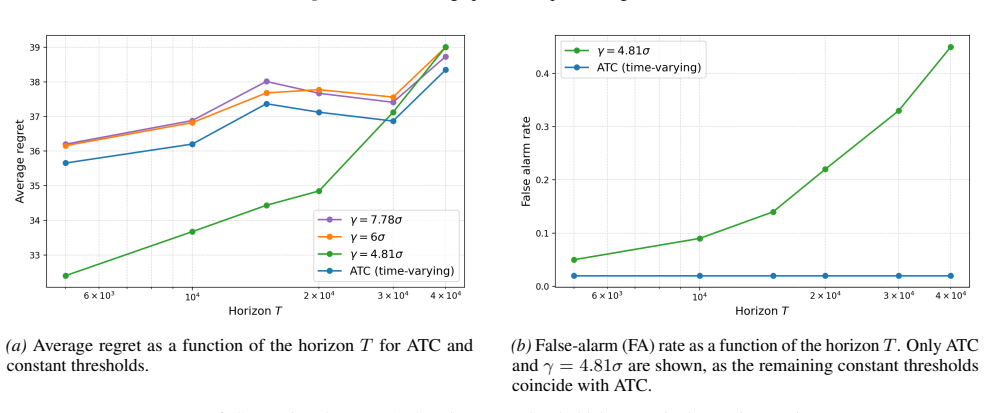
- [App. A.1.5] The sensitivity experiment shows that when σ is underestimated by a factor of 2, ATC diverges due to excessive false alarms. This is a useful caveat; the main text says ATC "only requires knowledge of the sub-Gaussian proxy σ" without mentioning this fragility. A sentence acknowledging the misspecification sensitivity would strengthen the presentation.
- [§3.3 / Eq. (14)] As noted in the major comments, the M² term in Lemma 3.1 seems spurious. If intended as a universal bound under alarms, it needs a proof; otherwise it should be deleted or replaced with (M/σ)² if a dimensionless quantity is desired.
- [App. A.1.6] The informal bound R(t) ≤ min{aΔ², σ²(γ_t^r)²} is stated without derivation. While it is illustrative, it would be helpful to state that this is an informal heuristic and not a formal inequality for the cumulative regret up to time t.
Circularity Check
No circular derivation: ATC threshold is derived from concentration inequalities; the lower bound is an independent two-point/van Trees argument; the only flagged issue is a missing M≥cσ qualification in Thm 4.2, which is a correctness gap, not circularity.
full rationale
The derivation chain is self-contained. ATC's threshold γ^r_t is obtained in Lemma A.2 from a union-bound/Chernoff calculation (Eq. 36–39), not from fitting regret targets; the algorithm's regret upper bound then follows by the decomposition Lemma A.1, the confidence bound, and the bias/variance lemmas A.3–A.5. The key SNR-degradation bound Lemma 3.1 is proven as an algebraic inequality (Claim A.12) for the two-change case and extended by compressing the prefix to a mean μ0; the only caveat is footnote 6's admission that other splits may dominate, which is an acknowledged proof-tightness issue rather than circularity. The lower bound (Thm 4.2) is built on a data-processing two-point argument (Claim A.7, Lemma A.9) and a van Trees Bayes–minimax variance bound (Lemma A.10), neither of which uses ATC or its threshold, so the near-minimax claim is not derived from the upper bound. The self-citations (e.g., Besbes et al. 2015) are background references for dynamic regret and are not load-bearing. The manuscript does contain a flagged limitation in App. A.5 ('For simplicity, we assume M > cσ when deriving the variance lower bound') that is absent from the statement of Thm 4.2; this is a correctness/qualification concern about small M, not a circular derivation. No prediction is fitted and no fitted value is renamed as a prediction.
Assumptions & free parameters
free parameters (4)
- α (detection error budget) =
0.05 in all experiments
- σ (sub-Gaussian variance proxy) =
σ=1 (synthetic); σ=1, 'estimated offline from the data and yields the best empirical performance' (NAB, App. A.1.5)
- b (multiscale grid factor in the efficient variant) =
b=2
- NAB ground-truth change points =
{377, 420, 592, 3575}
assumptions (5)
- domain assumption Observations are independent and (X_t − μ_t) is sub-Gaussian with known proxy σ² (Section 2).
- domain assumption Mean diameter is bounded: max|μ_u − μ_v| ≤ M (Eq. 1), with M unknown to the learner.
- domain assumption The mean is piecewise constant with change points 1=τ₀<τ₁<...<τ_S<τ_{S+1}=T+1; no detectability or spacing assumptions (Section 2).
- ad hoc to paper Variance lower bound assumes M ≥ c₀σ (App. A.5.3); stated in the proof but not in the statement of Theorem 4.2.
- ad hoc to paper Lemma 3.1's proof assumes ATC raises no alarm in (r, τ_j] (App. A.6); the lemma as stated is broader than the proven case.
Cite this review
Pith. "Pith review of The Cost of Learning Under Multiple Change Points." pith.science (2026). https://pith.science/paper/QXMKQVDV
@misc{pith2026260211406,
  author       = {Pith},
  title        = {Pith review of: The Cost of Learning Under Multiple Change Points},
  year         = {2026},
  howpublished = {\url{https://pith.science/paper/QXMKQVDV}},
  note         = {Machine review of arXiv:2602.11406}
}
read the original abstract
We consider an online learning problem in environments with multiple change points. In contrast to the single change point problem that is widely studied using classical "high confidence" detection schemes, the multiple change point environment presents new learning-theoretic and algorithmic challenges. Specifically, we show that classical methods may exhibit catastrophic failure (high regret) due to a phenomenon we refer to as endogenous confounding. To overcome this, we propose a new class of learning algorithms dubbed Anytime Tracking CUSUM (ATC). These are horizon-free online algorithms that implement a selective detection principle, balancing the need to ignore "small" (hard-to-detect) shifts, while reacting "quickly" to significant ones. We prove that the performance of a properly tuned ATC algorithm is nearly minimax-optimal; its regret is guaranteed to closely match a novel information-theoretic lower bound on the achievable performance of any learning algorithm in the multiple change point problem. Experiments on synthetic as well as real-world data validate the aforementioned theoretical findings.
Figures


Figures from the paper (8 more)




Reference graph
Works this paper leans on
-
[2]
yields a regret lower bound of order σ2 logT. Hence, in what follows we restrict attention to policies for which there exists a window indexj∈[m]such that q:=P ∞(Aj)≤ α m .(65) We viewqas quantifying the stability of the policy on windowW j under the ”no-change” instance. Step 3 - Information constraint (stability limits adaptivity).We now consider the en...
2008
-
[6]
X t∈Bm ˆµr t −¯µr t 2 Fr # =E
The statistic at the split k⋆ =τ j and timet max is (Dr(j) k⋆,tmax )2 = 1 σ2 a(j) L Bj a(j) L +B j ∆(eff) j 2 ,(50) 4Specifically, we use Pm b=1 a2 (a+b)2 ≤ R m 0 a2 (a+x)2 dx= am a+m . 5In the derivation below we compute the regret at the edge pointt=τ j separately to ensurek ⋆ < t. 6If τj−1 was detected, the split k⋆ =τ j maximizes the population contra...
1991
-
[2010]
Crafting papers on machine learning
Langley, P. Crafting papers on machine learning. In Langley, P. (ed.),Proceedings of the 17th International Conference on Machine Learning (ICML 2000), pp. 1207–1216, Stanford, CA,
2000
-
[2016]
Garivier, A. and Moulines, E. On upper-confidence bound policies for non-stationary bandit problems.arXiv preprint arXiv:0805.3415,
-
[2018]
Procedures for reacting to a change in distribution.The annals of mathematical statistics, pp
Lorden, G. Procedures for reacting to a change in distribution.The annals of mathematical statistics, pp. 1897–1908,
1908
-
[2024]
Huang, Y .-H. and Veeravalli, V . V . Sequential change detection for learning in piecewise stationary bandit environments. arXiv preprint arXiv:2501.10974,
Reviewed August 3, 2026 · model on record in the stance chip above.
Discussion (0). Continue with ORCID to comment.