High-Order Implicit Low-Rank Method with Spectral Deferred Correction for Matrix Differential Equations

Shun Li; Yan Jiang; Yingda Cheng

REVIEW 4 major objections 6 minor 1 cited by

High-Order Implicit Low-Rank Method with Spectral Deferred Correction for Matrix Differential Equations

T0 review · 4 major / 6 minor · reviewed 2026-08-11 · deepseek-v4-flash

Challenge this review Re-run · record.json Download PDF Read on arXiv ↗ Review JSON

Pith's one-line read This paper proves that spectral deferred correction can raise the first-order merge-BUG low-rank integrator to any chosen temporal order, with level-dependent truncation tolerances and without K/L subspace solves in the correction passes.

desk verdict Publishable after revision: SDC-mBUG is a genuinely new combination with confirmed orders on smooth, non-stiff tests, but Theorem 3.2's Lipschitz-only hypotheses don't deliver the claimed O(h^{K+2}) error. read the letter →

arxiv 2412.09400 v1 pith:ROGLZXAC submitted 2024-12-12 math.NA cs.NA

Shun Li , Yan Jiang , Yingda Cheng This is my paper · ORCID

classification math.NAcs.NA MSC 65L0565L2065M20

keywords dynamiclow-rankapproximationspectraldeferredcorrectionmerge-BUGmethodmatrixdifferentialequationsimplicitsoftthresholdinghardtruncationadvection-diffusionequation

verification ladder T0 review T1 audit T2 compute T3 formal

The pith

A machine-rendered reading of the paper's core claim, the machinery that carries it, and where it could break.

The reading

This paper proposes a way to give dynamic low-rank time integrators high-order temporal accuracy without abandoning their low-rank storage: wrap the first-order merge-BUG (mBUG) scheme in spectral deferred correction (SDC). For linear matrix differential equations whose solutions stay approximately low-rank, the resulting SDC-mBUG scheme is proven to achieve (K+1)th-order local accuracy under standard Lipschitz and boundedness assumptions, provided the time step satisfies hL<1. The proof also shows that truncation tolerances can grow with early correction levels, lowering intermediate ranks, and that the correction passes can skip the expensive K- and L-subspace solves. Numerical tests on advection-diffusion and Schrödinger-type problems confirm the predicted orders; soft thresholding is shown to track solution rank better for weakly or non-dissipative problems, while hard thresholding can be more accurate when singular values decay abruptly.

What carries the argument

The machinery is SDC applied to the Picard integral equation with mBUG as the base integrator: after a first-order mBUG sweep, each correction level solves for a low-rank approximation to the Picard equation, with the residual integral precomputed by interpolatory quadrature and truncated to tolerance $epsilon_r^{{(k)}}$. The S-step projects onto the span of the previous solution, current F values, and the residual, while K/L solves are dropped, relying on the Neumann-series view of SDC. The induction quantity $delta^{{(k+1)}}$=O(h $delta^{{(k)}}$ + $epsilon_s^{{(k+1)}}$ + h $epsilon_f^{{(k)}}$ + $epsilon_r^{{(k)}}$) is what carries the order improvement from one correction level to the next.

What would settle it

Run the scheme on a stiff linear test such as X'=-$\lambda$ X, or a stiff advection-diffusion discretization, with a fixed time step h satisfying h $\lambda$ > 1, and check whether the local error still follows O($h^{{K+2}}$); since the theorem's hL<=gamma<1 assumption no longer holds, order loss or instability would show the proof's regime is genuinely restrictive.

Watch

Extended reading notes

Core claim

The central claim is Theorem 3.2: starting from the first-order mBUG method, K SDC correction levels with P subintervals give the local error bound ||X_{n+1}-X(t_{n+1})|| <= C_{K+1}($delta^{{(K+1)}}$ + $h^{{min(K+2,P+2)}}$), with $delta^{{(1)}}$=O(epsilon_s+epsilon_f h) and $delta^{{(k+1)}}$=O(h $delta^{{(k)}}$ + $epsilon_s^{{(k+1)}}$ + h $epsilon_f^{{(k)}}$ + $epsilon_r^{{(k)}}$). Under the tolerance schedule epsilon_s=O($h^{2}$), epsilon_f=O(h), $epsilon_s^{{(k+1)}}$=$epsilon_r^{{(k)}}$=O($h^{{k+2}}$), $epsilon_f^{{(k)}}$=O($h^{{k+1}}$), and with P=K, this yields O($h^{{K+2}}$) local error, i.e. (K+1)th-order temporal convergence. The argument proceeds by induction on the correction level, so each correction reduces the dominant error by one power of h. The method's design rests on two efficiency choices the theory supports: level-dependent truncation tolerances and omission of K/L steps in the corrections, leaving only a small Galerkin S-step.

Load-bearing premise

The proof leans on two premises: the first-order error bound of the base mBUG method, and the small-step condition hL<1 that keeps the (1-hL) factors positive; if either fails, the induction collapses.

Editorial extensions

If this is right

With P=K and the stated tolerance schedule, the SDC-mBUG scheme attains (K+1)th-order temporal accuracy, so any desired order can be selected by adding correction levels.
Larger truncation tolerances are permitted at early correction levels, which reduces the intermediate numerical rank and computational cost without damaging the final order.
The correction passes avoid inverting large Sylvester systems from the K- and L-steps, needing only the small linear system from the Galerkin S-step.
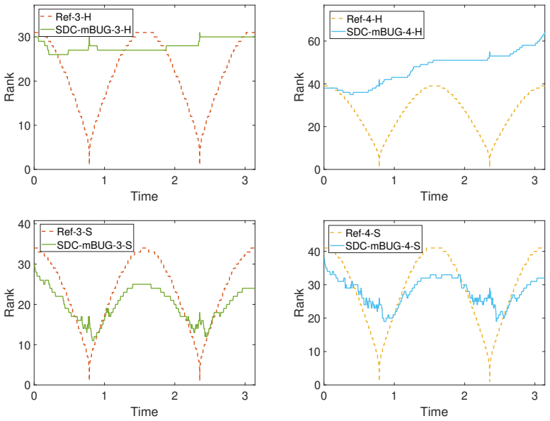
Soft thresholding offers better rank control for weakly or non-dissipative problems with smoothly decaying singular values, while hard thresholding can give smaller errors when the singular value sequence decays abruptly.
The theoretical bound applies to all Lipschitz continuous and bounded right-hand sides of the stated linear matrix equation form, not just the numerical examples tested.

Reading between the lines

Editorial extensions of the paper, not claims the author makes directly.

A natural extension left implicit by the paper is testing whether the level-dependent tolerance schedule can be adapted to stiff problems where hL is not small, since the current proof requires hL<1.
The subspace choice that omits K/L steps is motivated by viewing SDC as a preconditioned Neumann series; the same deferred-correction strategy could plausibly be wrapped around other low-rank base integrators, such as midpoint or DIRK-based BUG variants.
Soft thresholding's non-expansiveness, which the paper uses only numerically, may support a rigorous rank-control statement beyond the observed experiments.
The proof is developed for linear matrix differential equations; a testable extension is whether the same order and tolerance analysis survives nonlinear right-hand sides or tensor-valued unknowns.

Share X Bluesky LinkedIn Reddit HN

Editorial analysis

A structured set of objections, weighed in public.

Desk editor's note, referee report, and a circularity audit.

Desk Editor's Note

read the letter

Dear colleague,

The short version: this is a real contribution. The paper wraps spectral deferred correction around the mBUG low-rank integrator, and it adds two practical improvements: level-dependent truncation tolerances that keep intermediate ranks low, and a K/L-free correction step that avoids the expensive linear solves from the BUG framework. The numerical results are honest and the observed convergence orders match the intended order for smooth, non-stiff problems. I would send it to review, but the main theorem needs fixing before I trust it as stated.

What is new and what works. The SDC-mBUG combination does not appear in the earlier high-order low-rank literature (midpoint, DIRK, IMEX, Krylov enrichment), so the method is novel. The level-dependent tolerance analysis is genuinely useful: it shows that early correction levels can tolerate looser truncation, and that is what controls the intermediate rank. Omitting the K- and L-steps in the corrections is a meaningful cost saving, and the proof of the subspace choice is clean. The hard-versus-soft truncation comparison is a nice addition; the rank plots support the claim that soft thresholding tracks smooth singular value decay better.

Soft spots, in order of magnitude. First, Theorem 3.2 is internally inconsistent. The proof asserts that the quadrature error of the interpolated Picard integral is O(h^{P+2}) (term (A)), but that estimate requires F(X(t),t) to be sufficiently smooth in t. Under the stated Lipschitz-only hypothesis, polynomial interpolation of a Lipschitz function on an interval of length h gives at best O(h^2) integral error, independent of P. Section 2.3 explicitly says SDC assumes F is sufficiently smooth, so the theorem's Lipschitz-only statement is not supported by its own proof. This is patchable, not fatal: add a smoothness assumption to Theorem 3.2 and the induction goes through. Second, the bound-ness assumption ||F|| <= B does not hold for the linear model (1) when A is nonzero; a local boundedness argument on the tube around the solution would be the standard fix. Third, the condition hL <= gamma < 1 excludes the stiff regime, yet the introduction motivates implicit methods precisely for stiffness. The tests are all smooth and non-stiff, so the paper does not demonstrate the stiffness robustness it advertises. Fourth, Lemma 3.1, the base case of the induction, comes from an unpublished preprint by one of the authors; a referee will want that result restated or at least a stable version of the preprint. Finally, there is no comparison with existing high-order low-rank integrators and no code shipped.

Who this is for: numerical analysts working on low-rank time integration for matrix ODEs. They will find the SDC-mBUG construction worth studying, and the soft-thresholding rank-control experiments are a useful data point. It deserves a serious referee, but the referee should ask for a corrected theorem statement and ideally a stiff test case.

Best, [Your name]

Referee Report

4 major / 6 minor

Summary. The manuscript proposes an SDC-based high-order temporal integrator for linear matrix differential equations in low-rank format. It combines the first-order merge-BUG (mBUG) scheme with spectral deferred correction, deriving a level-dependent truncation tolerance strategy and a subspace construction that avoids the costly K/L steps in the correction sweeps. The main result, Theorem 3.2, gives a local error bound of the form O(delta^(K+1) + h^{min(K+2,P+2)}) under Lipschitz and boundedness assumptions. Numerical experiments on a manufactured solution, a Schrödinger equation, anisotropic diffusion, and pure rotation confirm the expected orders for K=2,3,4 and compare hard versus soft thresholding for rank control.

Significance. If the theorem's hypotheses are corrected, the scheme is a useful extension of mBUG to high order, with a carefully designed tolerance hierarchy and a cheaper correction step. The paper's strengths are the detailed truncation-error scaling analysis in Section 3.1 and Remark 3.1, the explicit avoidance of K/L solves in the correction steps, and the clean convergence tables and rank-evolution plots in Section 4. However, the central error bound as stated does not follow from the stated assumptions, and the assumptions exclude the stiff, linear model that motivates the method; these issues must be fixed before the main claim can be accepted.

major comments (4)

[Section 3.2, proof of Theorem 3.2, term (A)] The estimate ||(A)|| <= C_A h^{P+2} for the quadrature error of the Picard integral is asserted without any smoothness hypothesis. Assumption (12) gives only Lipschitz continuity and boundedness; for a merely Lipschitz integrand on an interval of length h, the polynomial interpolation error is at best O(h) and the integral error is only O(h^2) regardless of P. Consequently the induction in (14) cannot produce the claimed order min(K+2,P+2), and Theorem 3.2 as stated is internally inconsistent with Section 2.3, which explicitly assumes F is sufficiently smooth. The theorem and Remark 3.1 need an explicit smoothness assumption (e.g., F and the exact solution are sufficiently differentiable on the time interval) or a revised argument that derives high order from a weaker regularity condition; the numerical tests use smooth data and cannot close this gap.
[Section 3.2, Eq. (12)] The global boundedness assumption ||F(X,t)|| <= B is incompatible with the linear format (1) whenever any A_j is nonzero, since ||sum_j A_j X B_j^T + G(t)|| is unbounded as ||X|| tends to infinity. Thus Theorem 3.2 does not apply to the model equation that motivates the paper. Replace the global bound with a local bound on a tube around the exact solution, or with boundedness of the exact solution and of F on its range, and verify that the mBUG base bound in Lemma 3.1 remains valid under that replacement.
[Section 3.2, Lemma 3.1 and Theorem 3.2] The base case of the SDC induction is the first-order mBUG local error bound from the unpublished preprint [1], and Lemma 3.1 is stated without proof. Since this lemma supplies delta^(1)=O(eps_s + eps_f h) and the proof of (14) relies on it, the manuscript should make this result self-contained, or quote a precise theorem with a full proof in an appendix. This is not a cosmetic issue: a gap in the base case directly invalidates the induction.
[Introduction and Theorem 3.2] The paper motivates implicit methods by stiffness ('Equation (1) is assumed to be stiff to necessitate implicit methods'), but the theorem requires hL <= gamma < 1, so for large Lipschitz constant L the result only applies for impractically small steps. The numerical experiments in Tables 1-4 are non-stiff and all use smooth, low-rank solutions; no stiff example is included. The claims should either be restricted to non-stiff regimes, or the analysis and experiments should directly address the stiff case, for example with a problem-independent or contractivity-based bound and a stiff numerical test.

minor comments (6)

[Section 3.2, final displayed equation in the proof] The indices 'P+1' should be 'P', i.e., X^{(K+1)}_{n,P} - X(t_{n,P}); as written the expression refers to a node t_{n,P+1} that does not exist.
[Section 3.2, Eq. (12)] The second Lipschitz term is written L|s-z|; it should be L|s-t| to match the arguments (Y,s) and (Z,t).
[Section 2.3, Theorem 2.1 and following Remark] The local error is stated as O(h^{min(K+2,P+2)}), while the remark states the order is min(K+1,P+1); clarify that the former is local and the latter global.
[Section 3.2, Theorem 3.2 and Remark 3.1] The exponent notation 'hmin' should be rendered as h^{min(...)}; the inline notation is ambiguous in several places.
[Section 3.1 and Section 4] There is a typo 'optimial accuracy' after Step C-3, and the constant C in the numerical tolerance formula is introduced without saying how it was chosen or whether the observed convergence rates depend on that choice.
[Section 4] The reference solutions in Examples 2-4 are computed on a finer spatial grid than the numerical solutions, but spatial and temporal errors are not separated; a brief statement confirming that spatial error is negligible would strengthen the convergence tables.

Circularity Check

0 steps flagged · score 2.0 of 10

No significant circularity: the SDC-mBUG high-order error bound is proved by induction from a cited first-order mBUG base case, not by assuming its own conclusion.

full rationale

Theorem 3.2 does not assume the claimed high-order accuracy. Its proof derives the error recursion δ^{(k+1)} = O(h δ^{(k)} + ε_s^{(k+1)} + hε_f^{(k)} + ε_r^{(k)}) from the Picard integral error terms (A), (B), (C) and the truncation inequalities (15) and (16), and the final O(h^{K+2}) order follows only after inserting the explicit tolerance scaling ε_s=O(h^2), ε_f=O(h), ε_s^{(k+1)}=ε_r^{(k)}=O(h^{k+2}), ε_f^{(k)}=O(h^{k+1}). This is a genuine derivation, not an identity with the conclusion. The only same-author dependency is Lemma 3.1, which imports the first-order mBUG error bound from [1] (Appelö and Cheng) as the base case of the induction; although this is load-bearing for the proof, it is a standard citation of prior work on a different (first-order) scheme, and the high-order SDC correction content is newly derived here. The numerical experiments compare against full-rank RK4 reference solutions and independently confirm the predicted orders, so the accuracy claim is not manufactured by the tolerance choices. A reviewer concern that the O(h^{P+2}) interpolation estimate in term (A) requires more smoothness than the Lipschitz assumption (12) provides is a correctness or robustness gap, not circularity. Overall, no step reduces by construction to its own input, so the circularity score is low.

Assumptions & free parameters 2 free parameters · 4 assumptions · 0 invented entities

The proof pulls in standard DLRA and SDC background (projection, truncation operators, Picard integral) plus two domain assumptions: global Lipschitz/bounded F and small-step hL<1. No new physical entities are introduced.

free parameters (2)

truncation tolerances epsilon_s, epsilon_f, epsilon_s^{(k+1)}, epsilon_r^{(k)}, epsilon_f^{(k)} = epsilon_s=O(h^2), epsilon_f=O(h), epsilon_s^{(k+1)}=epsilon_r^{(k)}=O(h^{k+2}), epsilon_f^{(k)}=O(h^{k+1})
Hand-chosen algorithmic tolerances required by the error recurrence in Theorem 3.2; they are not fitted to match solution data, but their scaling is assumed in the proof.
constant C in numerical tolerance formula = 2 (4*pi/Nx + 4*pi/Ny)^{-1}
Hand-selected multiplier in the experiments (Section 4); it absorbs the spatial mesh scale and is not optimized against the exact solutions.

assumptions (4)

domain assumption F is globally Lipschitz in both variables and bounded: ||F(Y,s)-F(Z,t)|| <= L||Y-Z|| + L|s-t| and ||F(X,t)|| <= B.
Invoked in Section 3.2, Eq. (12), to prove the local truncation error theorem; excludes stiff and unbounded growth cases.
domain assumption Small time step condition hL <= gamma < 1.
Used in the proofs of Lemma 3.1 and Theorem 3.2 to invert (1-hL) factors; does not cover the stiff regime.
standard math The low-rank truncation operators satisfy rank(T_epsilon(X)) <= rank(X) and ||X - T_epsilon(X)|| <= epsilon.
Section 2.1 defines T_epsilon as satisfying these properties; hard and soft thresholding both satisfy them.
standard math Spectral deferred correction collocation quadrature weights {w_{m,s}} yield interpolation error O(h^{P+2}).
Standard SDC theory from [9]; used in bounding term (A) in the proof.

how reviews work

0 comments

Cite this review

Pith. "Pith review of High-Order Implicit Low-Rank Method with Spectral Deferred Correction for Matrix Differential Equations." pith.science (2026). https://pith.science/paper/ROGLZXAC

@misc{pith2026241209400,
  author       = {Pith},
  title        = {Pith review of: High-Order Implicit Low-Rank Method with Spectral Deferred Correction for Matrix Differential Equations},
  year         = {2026},
  howpublished = {\url{https://pith.science/paper/ROGLZXAC}},
  note         = {Machine review of arXiv:2412.09400}
}

read the original abstract

In this paper, we develop a low-rank method with high-order temporal accuracy using spectral deferred correction (SDC) to compute linear matrix differential equations. In [1], a low rank numerical method is proposed to correct the modeling error of the basis update and the Galerkin (BUG) method, which is a computational approach for DLRA. This method (merge-BUG/mBUG method) has been demonstrated to be first order convergent for general advection-diffusion problems. In this paper, we explore using SDC to elevate the convergence order of the mBUG method. In SDC, we start by computing a first-order solution by mBUG, and then perform successive updates by computing low-rank solutions to the Picard integral equation. Rather than a straightforward application of SDC with mBUG, we propose two aspects to improve computational efficiency. The first is to reduce the intermediate numerical rank by detailed analysis of dependence of truncation parameter on the correction levels. The second aspect is a careful choice of subspaces in the successive correction to avoid inverting large linear systems (from the K- and L-steps in BUG). We prove that the resulting scheme is high-order accurate for the Lipschitz continuous and bounded dynamical system. We consider numerical rank control in our framework by comparing two low-rank truncation strategies: the hard truncation strategy by truncated singular value decomposition and the soft truncation strategy by soft thresholding. We demonstrate numerically that soft thresholding offers better rank control in particular for higher-order schemes for weakly (or non-)dissipative problems.

Figures

Figures reproduced from arXiv: 2412.09400 by the authors.

**Figure 1.** Example 1. The rank evolution of the numerical solutions obtained by the SDC-mBUG schemes over time is shown, where the dashed line represents the rank evolution of the reference solution. Top: hard truncation; bottom: soft truncation. Left: the third-order SDC-mBUG scheme; right: the fourth-order SDC-mBUG scheme. 16 [PITH_FULL_IMAGE:figures/full_fig_p016_1.png] view at source ↗

**Figure 2.** Example 2. The rank evolution of the numerical solutions obtained by the SDC-mBUG schemes over time is shown, where the dashed line represents the rank evolution of the reference solution. Top: hard truncation; bottom: soft truncation. Left: the third-order SDC-mBUG scheme; right: the fourth-order SDC-mBUG scheme. 18 [PITH_FULL_IMAGE:figures/full_fig_p018_2.png] view at source ↗

**Figure 3.** Example 3. The rank evolution of the numerical solutions obtained by the SDC-mBUG schemes over time is shown, where the dashed line represents the rank evolution of the reference solution. Top: hard truncation; bottom: soft truncation. Left: the third-order SDC-mBUG scheme; right: the fourth-order SDC-mBUG scheme [PITH_FULL_IMAGE:figures/full_fig_p020_3.png] view at source ↗

Figures from the paper (1 more)

**Figure 4.** Figure 4: Example 4. The rank evolution of the numerical solutions obtained by the SDC-mBUG schemes over time is shown, where the dashed line represents the rank evolution of the reference solution. Top: hard truncation; bottom: soft truncation. Left: the third-order SDC-mBUG sc…

Discussion (0). Continue with ORCID to comment.

Forward citations

Cited by 1 Pith paper

Reviewed papers in the Pith corpus that reference this work. Sorted by Pith novelty score. Full citation record

Iterative thresholding low-rank time integration
math.NA 2025-07 conditional novelty 7.0 of 10

Iterative soft thresholding is combined with collocation-based time stepping to produce low-rank solutions of evolution equations whose ranks stay quasi-optimal for the achieved accuracy.

Reference graph

Works this paper leans on

25 extracted references · 22 canonical work pages · cited by 1 Pith paper

[1]

Robust Implicit Adaptive Low Rank Time-Stepping Methods for Matrix Differential Equations

D. Appel¨ o and Y. Cheng. Robust implicit adaptive low rank time-ste pping methods for matrix diﬀerential equations. arXiv preprint arXiv:2402.05347 , 2024

work page Pith review arXiv 2024
[2]

Bachmayr

M. Bachmayr. Low-rank tensor methods for partial diﬀerentia l equations. Acta Numerica , 32:1–121, 2023

work page 2023
[3]

Bachmayr and R

M. Bachmayr and R. Schneider. Iterative methods based on sof t thresholding of hierarchical tensors. Foundations of Computational Mathematics , 17:1037–1083, 2017

work page 2017
[4]

J.-F. Cai, E. J. Cand` es, and Z. Shen. A singular value thresholdin g algorithm for matrix completion. SIAM Journal on optimization , 20(4):1956–1982, 2010

work page 1956
[5]

Ceruti, L

G. Ceruti, L. Einkemmer, J. Kusch, and C. Lubich. A robust seco nd-order low-rank BUG integrator based on the midpoint rule. BIT Numerical Mathematics , 64(3):30, 2024

work page 2024
[6]

Ceruti, J

G. Ceruti, J. Kusch, and C. Lubich. A rank-adaptive robust inte grator for dynamical low-rank approximation. BIT Numerical Mathematics , 62(4):1149–1174, 2022

work page 2022
[7]

Ceruti and C

G. Ceruti and C. Lubich. An unconventional robust integrator for dynamical low-rank approx- imation. BIT Numerical Mathematics , 62(1):23–44, 2022

work page 2022
[8]

Christlieb, B

A. Christlieb, B. Ong, and J.-M. Qiu. Integral deferred correct ion methods constructed with high order Runge–Kutta integrators. Mathematics of Computation , 79(270):761–783, 2010

work page 2010

Show all 25 references

[9]

A. Dutt, L. Greengard, and V. Rokhlin. Spectral deferred cor rection methods for ordinary diﬀerential equations. BIT Numerical Mathematics , 40:241–266, 2000. 22

2000
[10]

El Kahza, W

H. El Kahza, W. Taitano, J.-M. Qiu, and L. Chac´ on. Krylov-bas ed adaptive-rank implicit time integrators for stiﬀ problems with application to nonlinear Fokke r-Planck kinetic models. Journal of Computational Physics , 518:113332, 2024

2024
[11]

Grasedyck, D

L. Grasedyck, D. Kressner, and C. Tobler. A literature surve y of low-rank tensor approximation techniques. GAMM-Mitteilungen, 36(1):53–78, 2013

2013
[12]

Hackbusch

W. Hackbusch. Tensor spaces and numerical tensor calculus , volume 42. Springer, 2012

2012
[13]

Hagstrom and R

T. Hagstrom and R. Zhou. On the spectral deferred correct ion of splitting methods for ini- tial value problems. Communications in Applied Mathematics and Computational S cience, 1(1):169–205, 2007

2007
[14]

Hiriart-Urruty and C

J.-B. Hiriart-Urruty and C. Lemar´ echal. Convex analysis and minimization algorithms I: Fundamentals, volume 305. Springer science & business media, 1996

1996
[15]

Huang, J

J. Huang, J. Jia, and M. Minion. Accelerating the convergence o f spectral deferred correction methods. Journal of Computational Physics , 214(2):633–656, 2006

2006
[16]

B. N. Khoromskij. Tensor numerical methods in scientiﬁc computing , volume 19. Walter de Gruyter GmbH & Co KG, 2018

2018
[17]

Kieri, C

E. Kieri, C. Lubich, and H. Walach. Discretized dynamical low-ran k approximation in the presence of small singular values. SIAM Journal on Numerical Analysis , 54(2):1020–1038, 2016

2016
[18]

Koch and C

O. Koch and C. Lubich. Dynamical low-rank approximation. SIAM Journal on Matrix Analysis and Applications, 29(2):434–454, 2007

2007
[19]

H. Y. Lam, G. Ceruti, and D. Kressner. Randomized low-rank Ru nge-Kutta methods. arXiv preprint arXiv:2409.06384, 2024

2024 arXiv
[20]

A. T. Layton and M. L. Minion. Conservative multi-implicit spectra l deferred correction methods for reacting gas dynamics. Journal of Computational Physics , 194(2):697–715, 2004

2004
[21]

S. Meng, D. Appelo, and Y. Cheng. Preconditioning Low Rank Gen eralized Minimal Residual Method (GMRES) for Implicit Discretizations of Matrix Diﬀerential Eq uations. arXiv preprint arXiv:2410.07465, 2024

2024 arXiv
[22]

M. Minion. A hybrid parareal spectral deferred corrections m ethod. Communications in Applied Mathematics and Computational Science , 5(2):265–301, 2011

2011
[23]

M. L. Minion. Semi-implicit spectral deferred correction method s for ordinary diﬀerential equations. Communications in Mathematical Sciences , 1:471–500, 2003

2003
[24]

Nakao, J.-M

J. Nakao, J.-M. Qiu, and L. Einkemmer. Reduced Augmentation I mplicit Low-rank (RAIL) in- tegrators for advection-diﬀusion and Fokker-Planck models. arXiv preprint arXiv:2311.15143 , 2023

2023 arXiv
[25]

L. N. Trefethen. Spectral methods in MATLAB . SIAM, 2000. 23

2000

Pith tools

Reviewed August 11, 2026 · model on record in the stance chip above.

[1] [1]

Robust Implicit Adaptive Low Rank Time-Stepping Methods for Matrix Differential Equations

D. Appel¨ o and Y. Cheng. Robust implicit adaptive low rank time-ste pping methods for matrix diﬀerential equations. arXiv preprint arXiv:2402.05347 , 2024

work page Pith review arXiv 2024

[2] [2]

Bachmayr

M. Bachmayr. Low-rank tensor methods for partial diﬀerentia l equations. Acta Numerica , 32:1–121, 2023

work page 2023

[3] [3]

Bachmayr and R

M. Bachmayr and R. Schneider. Iterative methods based on sof t thresholding of hierarchical tensors. Foundations of Computational Mathematics , 17:1037–1083, 2017

work page 2017

[4] [4]

J.-F. Cai, E. J. Cand` es, and Z. Shen. A singular value thresholdin g algorithm for matrix completion. SIAM Journal on optimization , 20(4):1956–1982, 2010

work page 1956

[5] [5]

Ceruti, L

G. Ceruti, L. Einkemmer, J. Kusch, and C. Lubich. A robust seco nd-order low-rank BUG integrator based on the midpoint rule. BIT Numerical Mathematics , 64(3):30, 2024

work page 2024

[6] [6]

Ceruti, J

G. Ceruti, J. Kusch, and C. Lubich. A rank-adaptive robust inte grator for dynamical low-rank approximation. BIT Numerical Mathematics , 62(4):1149–1174, 2022

work page 2022

[7] [7]

Ceruti and C

G. Ceruti and C. Lubich. An unconventional robust integrator for dynamical low-rank approx- imation. BIT Numerical Mathematics , 62(1):23–44, 2022

work page 2022

[8] [8]

Christlieb, B

A. Christlieb, B. Ong, and J.-M. Qiu. Integral deferred correct ion methods constructed with high order Runge–Kutta integrators. Mathematics of Computation , 79(270):761–783, 2010

work page 2010