REVIEW 5 major objections 6 minor 26 references
Reinforced Disentanglers on Random Unitary Circuits
T0 review · 5 major / 6 minor · reviewed 2026-08-12 · deepseek-v4-flash
Pith's one-line read The paper claims that targeted projective measurements found by reinforcement learning can fully disentangle random Clifford circuits with far fewer projections than random-measurement MIPT studies, and that the optimal placement has a…
desk verdict Nice RL framing for measurement placement, but the reward sign error reverses the intended objective and the headline claim lacks quantitative support. read the letter →
The pith
A machine-rendered reading of the paper's core claim, the machinery that carries it, and where it could break.
The reading
What carries the argument
The load-bearing object is the binary matrix $P$ of measurement positions, where $P_{ij}=1$ means a $Z$-projection is inserted at site $i$ between consecutive unitary layers. The state of the reinforcement-learning agent is this matrix, the action flips one bit to add or delete a measurement, and an episode ends when the averaged von Neumann entropy over all $N-1$ contiguous bipartitions vanishes. The sparse reward is $R = 1 - C/(F N)$, with $C=\sum_l f_{l;\alpha} m_l$ the layer-weighted measurement cost and $f_{l;\alpha}=2e^{-\alpha l}/(1+e^{-\alpha l})$ a monotone penalty that is small for early layers and large for late ones. Clifford and stabilizer simulation, through the Gottesman-Knill representation and the stabilizer formula for Rényi entropy, makes each entropy evaluation polynomial rather than exponential, which is what allows the PPO loop, a policy-gradient method with clipped updates, to search the configuration space.
What would settle it
Enumerate all $2^{N D/2}$ binary measurement configurations for the smallest circuits, such as $N=4$ and $D/2=3$, and find the least number of projections that makes the averaged von Neumann entropy vanish; if the true minimum is materially lower or higher than the PPO-reported count, the learned numbers are not the raw minimum.
Extended reading notes
Core claim
The central discovery claimed is that a PPO-trained agent finds a configuration of projections that makes the averaged von Neumann entropy over all contiguous bipartitions vanish exactly, meaning the final state is a product state, and that the number of projections in this configuration, averaged over episodes, is much smaller than the measurement counts used in MIPT numerics. The paper reports that this number scales linearly with the number of qubits, saturates as a hyperbolic tangent with circuit depth, and has a layer-resolved profile that shifts from late layers to earlier layers as the penalty slope increases. The authors take this as evidence that there is a learnable, structured efficient disentangler that random-projection studies do not see.
Load-bearing premise
The reported minimum measurement counts assume the trained policy converged to a near-optimal configuration and that minimizing the layer-weighted reward is the same as minimizing the raw number of projections.
Editorial extensions
If this is right
- For a fixed depth and penalty slope, the minimal number of projections grows linearly with qubit number, roughly one additional measurement per two added qubits.
- For a fixed system size, the minimal number of projections saturates as circuit depth grows, following the saturation of entanglement entropy in unmeasured circuits.
- The optimal measurement pattern is depth-dependent: with a flat penalty most projections sit on late layers, and as the penalty slope rises they move to earlier layers.
- Randomly placed measurement patterns overestimate how many projections are needed to fully disentangle a random Clifford circuit.
- The fully disentangled final state is a product state, since the averaged entropy over all contiguous bipartitions vanishes.
Reading between the lines
- Exact enumeration on small systems would settle whether the learned configurations are truly minimal; the paper does not report such a check.
- Because the reward weights measurements by layer, the reported counts are not unconstrained raw minima, and an unweighted reward could change the comparison with measurement-induced phase transition rates.
- If the structured patterns are robust, the same optimization could be tried on non-Clifford circuits or on specific target states, where stabilizer shortcuts are unavailable and the learned patterns would have to be tested directly.
- The shift of measurements toward earlier layers under a steeper penalty hints that late-layer measurements are the most efficient per measurement, an effect that could be quantified by removing one learned measurement at a time.
Editorial analysis
A structured set of objections, weighed in public.
Referee Report
Summary. The paper formulates the problem of disentangling a random Clifford brick-wall circuit by placing projective measurements between unitary layers, and solves it with proximal policy optimization (PPO). The agent acts on a binary matrix of measurement locations; the sparse reward is nonzero only when the final averaged von Neumann entropy vanishes, and otherwise equals one minus a layer-weighted measurement cost. The paper reports that the number of measurements M(N,D,alpha) is approximately linear in the number of qubits N and saturates as a tanh function of the depth D, and that the measurement pattern has a nontrivial layer profile controlled by the penalty slope alpha. Based on these numbers, the abstract claims that the number of measurements required to disentangle a random circuit is drastically less than the measurement rates used in measurement-induced phase transition (MIPT) numerics.
Significance. The core idea -- replacing random measurement patterns in MIPT studies by optimized, deliberately placed disentanglers -- is a worthwhile and potentially useful research direction. The stabilizer-formalism entropy calculation is standard and efficient, and framing the placement problem as an RL game is natural and clearly explained. If the results were validated, they would provide a concrete, falsifiable quantitative statement about the overhead of disentangling random Clifford circuits, and the learned patterns could inform the design of disentangling protocols. However, the current manuscript does not establish these claims: the reward function contains a sign inconsistency with the stated design goal, the reported M is the count of a weighted-cost optimum rather than an unconstrained minimum, no quantitative MIPT baseline is supplied, and the PPO solutions are not certified as optimal even on small instances. These issues are load-bearing because they affect the definition of the central quantity M and the headline comparison to MIPT.
major comments (5)
- [II.B.3, Eq. (12)] The weight function f_{l;alpha} = 2e^{-alpha l}/(1+e^{-alpha l}) is strictly decreasing in l for every alpha > 0, as Fig. 2 confirms. This contradicts the design statement in Eq. (11) that the weights are a monotonically increasing penalty rate as the layer gets deeper. Because C = sum_l f_l m_l in Eq. (10), the implemented reward makes measurements on later layers cheaper, so it encourages the trivial last-layer solution that the text says it is designed to avoid. Consequently the interpretation in Section III.A -- that larger alpha moves measurements away from later layers -- is opposite to the incentive encoded in the reward, and the reported M(N,D,alpha) is not produced by the objective described in the text.
- [II.B.3, Eqs. (10) and (13)] The sparse reward is R = 1 - C/(F N), so among successful disentanglers the agent minimizes the weighted cost C = sum_l f_l m_l, not the number of projections M. Unless all f_l are equal (which happens only at alpha=0), the number M(N,D,alpha) is not the minimal number of measurements required to disentangle the circuit; it is the count belonging to a weighted-cost optimum. The abstract and Section III.A treat M as the number of measurements 'required,' and compare it with MIPT measurement rates, but the comparison is between a weighted cost optimum and an unweighted per-site rate. This mismatch affects the central quantitative claim of the paper.
- [III.A and Appendix A] The headline claim that the number of measurements is 'drastically less than the numerical results of measurement-induced phase transition papers' is not supported by any quantitative baseline. The paper never states the critical measurement rate or the total measurement counts from the cited MIPT works for the same system sizes and circuit depths, nor does it define whether the comparison is per-site rate, total projections, or something else. Without this baseline, the abstract's central comparison is unverifiable.
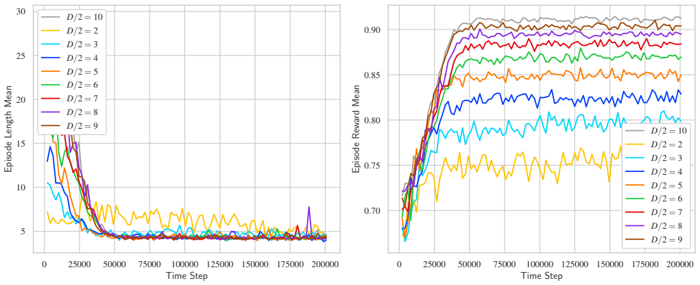
- [Appendix A and II.B.1] The PPO policies are not certified to be optimal or near-optimal. Training uses 2x10^5 to 5x10^5 time steps, and the learning curves in Figs. 6 and 7 show mean episode reward but no convergence criterion or comparison against an exact solution. For the smallest circuits (e.g., N=3-5, D/2=2-4) an exhaustive enumeration of all measurement subsets would be feasible and would provide a ground-truth check of Eq. (14). Without such a check, the quantities labeled 'min|R' are at best heuristic upper bounds rather than the 'required' numbers claimed in the abstract.
- [III.A, Eq. (21) and Fig. 5] The text states that 'the larger alpha is, the lesser the number of measurements placed on the later layers is,' but this is inconsistent with Eq. (12), where larger alpha makes later layers cheaper and should push measurements toward later layers. Figure 5 should be read carefully and the direction of the effect must be reconciled with the reward. As written, the textual claim, the equation, and the observed profile cannot all be correct; this directly undermines the paper's characterization of the pattern of optimal disentanglers.
minor comments (6)
- [Eq. (16)] The notation eta_{xi,xj} in Eq. (16) is introduced but never used anywhere else in the manuscript; either use it or remove it.
- [I, Acknowledgements] There are several typographical issues: 'Gottesmann' should be 'Gottesman', 'bipartions' in Eq. (9) should be 'bipartitions', and the author names contain garbled diacritics.
- [Eq. (14)] The notation 'min|R' in Eq. (14) is unclear. Please define precisely what the minimization is over (final configurations? policies? reward values?) and how the minimum is estimated from the PPO runs.
- [III.A and Table I] The table and Eq. (17) use inconsistent notation for the fit coefficients: Eq. (17) writes gamma^{N,alpha}_1(D) and gamma^{N,alpha}_2(D), while the text and Table I use gamma1 and gamma2 with different stated dependencies. Please make the notation uniform.
- [Table I caption] The caption says 'tanh and linear fit' but the table mixes two fit forms and two fitted quantities without clearly indicating which rows correspond to which form. A separate column or grouped layout would improve readability.
- [Appendix A] Reference [21] is an unpublished manuscript 'available upon request'; for reproducibility, please provide a public version or repository for the PyClifford package and the simulation code.
Circularity Check
No circularity found: the RL optimization is a genuine numerical search over a defined reward; the reported counts and patterns are not forced by construction or by self-citation.
full rationale
The paper's central quantities are the episode-averaged measurement counts M(N,D,α) obtained from a PPO agent trained with the sparse reward R=1-C/(FN) (Eqs. 10-14). This is an optimization over a hand-defined objective, not a derivation in which the output is algebraically identical to the input. The entanglement constraint (Eq. 9), the random Clifford dynamics, and the trained policy are independent ingredients; the reward weights alone do not determine whether a given configuration disentangles the state or how many measurements are needed. Hence the claim that optimized disentanglers use fewer measurements than random MIPT patterns is an empirical claim about the learned policy, not a tautology. There are no load-bearing self-citations: [21] is a software citation, and no uniqueness theorem is imported. However, the paper contains a serious internal inconsistency that is a correctness risk rather than circularity: Eq. (11) says the layer weights f_l should be monotonically increasing with depth, while the adopted f_{l;α}=2e^{-αl}/(1+e^{-αl}) in Eq. (12) is strictly decreasing for α>0. The reward therefore favors later-layer measurements, contrary to the stated design intent, and the qualitative interpretation in Sec. III.A that larger α moves measurements away from later layers is not supported by the reward's monotonicity. In addition, because R minimizes the weighted cost C rather than the raw projection count, M(N,D,α) is not automatically the unconstrained minimum claimed in the abstract. These are objective-mismatch and sign-error concerns, not cases where the result is equivalent to its inputs by construction.
Assumptions & free parameters
free parameters (5)
- Layer penalty slope α =
0.0 to 1.0 in scans; fixed at 0.1 for most runs
- Reward weight function f_{l;α} =
f_{l;α} = 2 e^{-α l} / (1 + e^{-α l})
- Fit coefficients γ1, γ2, γ3 in Eqs. (17)-(18) =
See Table I
- PPO hyperparameters (learning rate, entropy coefficient, time steps) =
lr inconsistent (0.1 vs 1e-3), ec=0.01, ts=2e5 to 5e5
- Unspecified reward scale pr =
50.0 in Figure 3 caption
assumptions (5)
- standard math Clifford circuits and stabilizer states can be simulated efficiently, and the von Neumann entropy of a stabilizer state is given by |A| - log2 |G_A| (Eq. 5).
- standard math Projective measurement of a single qubit in the σ_z basis on a stabilizer state yields another stabilizer state whose entanglement can be computed by the same formula.
- ad hoc to paper The reward function (13) with weights (12) correctly encodes the goal of 'efficient disentangling' (fewest projections while reaching a product state).
- ad hoc to paper A policy trained by PPO for 200,000 to 500,000 time steps reaches a near-optimal solution for the disentangling game.
- domain assumption The MIPT numerical results (random measurement rates) serve as the correct baseline for how many measurements are 'required' to disentangle.
Cite this review
Pith. "Pith review of Reinforced Disentanglers on Random Unitary Circuits." pith.science (2026). https://pith.science/paper/TC7DFCEG
@misc{pith2026241109784,
  author       = {Pith},
  title        = {Pith review of: Reinforced Disentanglers on Random Unitary Circuits},
  year         = {2026},
  howpublished = {\url{https://pith.science/paper/TC7DFCEG}},
  note         = {Machine review of arXiv:2411.09784}
}
read the original abstract
We search for efficient disentanglers on random Clifford circuits of two-qubit gates arranged in a brick-wall pattern, using the proximal policy optimization (PPO) algorithm \cite{schulman2017proximalpolicyoptimizationalgorithms}. Disentanglers are defined as a set of projective measurements inserted between consecutive entangling layers. An efficient disentangler is a set of projective measurements that minimize the averaged von Neumann entropy of the final state with the least number of total projections possible. The problem is naturally amenable to reinforcement learning techniques by taking the binary matrix representing the projective measurements along the circuit as our state, and actions as bit flipping operations on this binary matrix that add or delete measurements at specified locations. We give rewards to our agent dependent on the averaged von Neumann entropy of the final state and the configuration of measurements, such that the agent learns the optimal policy that will take him from the initial state of no measurements to the optimal measurement state that minimizes the entanglement entropy. Our results indicate that the number of measurements required to disentangle a random quantum circuit is drastically less than the numerical results of measurement-induced phase transition papers. Additionally, the reinforcement learning procedure enables us to characterize the pattern of optimal disentanglers, which is not possible in the works of measurement-induced phase transitions.
Figures


Figures from the paper (3 more)


Reference graph
Works this paper leans on
-
[1]
Proximal policy optimization Proximal Policy Optimization (PPO) [1] is a reinforce- ment learning algorithm designed to improve the stabil- ity and performance of policy gradient methods while (a) (b) FIG. 1. (a) Depiction of the random quantum circuits with the brick-wall structure. Random two-qubit Clifford gates are given in blue, and the projections a...
-
[2]
Rules of the disentangling game An environment is prepared by drawing a random Clif- ford circuit with circuit size N × D. We define the state space and the action space as the set of all possible N × D/2 binary matrices P by translating the length N disentangling circuit layers as length N bit-strings, see Figure 1. Thus, the binary matrix P is construct...
-
[3]
The sparse reward function is evaluated at the end of every episode
Rewards and penalties We design a sparse reward function. The sparse reward function is evaluated at the end of every episode. Placing the measurement on the last layer at least N/2 is the trivial solution. To avoid such trivial solutions, both reward functions consider the number of measure- ments needed to obtain non-trivial efficient disentanglers. Hen...
-
[4]
When the circuit gets deeper, and the averaged von Neumann entropy S in (9) stays the same or increases, one needs to increase the number of measurements at least one to keep the final state to be a product state. MN,α(D) saturates to a constant because there need no more additional measurements after the averaged von Neumann entropy SN,α(D) saturates to ...
-
[5]
J. Schulman, F. Wolski, P. Dhariwal, A. Radford, and O. Klimov, Proximal policy optimization algorithms (2017), arXiv:1707.06347 [cs.LG]
arXiv 2017
-
[6]
Nahum, J
A. Nahum, J. Ruhman, S. Vijay, and J. Haah, Phys. Rev. X 7, 031016 (2017)
2017
-
[7]
Skinner, J
B. Skinner, J. Ruhman, and A. Nahum, Phys. Rev. X 9, 031009 (2019)
2019
- [8]
Show all 26 references
-
[9]
A. Chan, R. M. Nandkishore, M. Pretko, and G. Smith, Phys. Rev. B 99, 224307 (2019)
2019
-
[10]
S. Choi, Y. Bao, X.-L. Qi, and E. Altman, Phys. Rev. Lett. 125, 030505 (2020)
2020
-
[11]
Breuer and F
H.-P. Breuer and F. Petruccione, The theory of open quantum systems (Oxford University Press, USA, 2002)
2002
-
[12]
Y. Li, X. Chen, and M. P. A. Fisher, Physical Review B 98, 10.1103/physrevb.98.205136 (2018)
2018 doi
-
[13]
A. Chan, R. M. Nandkishore, M. Pretko, and G. Smith, Physical Review B 99, 10.1103/physrevb.99.224307 (2019)
2019 doi
-
[14]
R. S. Sutton and A. G. Barto, Reinforcement Learning: An Introduction, 2nd ed. (The MIT Press, 2018)
2018
-
[15]
Gottesman, The heisenberg representation of quan- tum computers (1998), arXiv:quant-ph/9807006 [quant- ph]
D. Gottesman, The heisenberg representation of quan- tum computers (1998), arXiv:quant-ph/9807006 [quant- ph]
1998 arXiv
-
[16]
Hamma, R
A. Hamma, R. Ionicioiu, and P. Zanardi, Physical Review A 71, 10.1103/physreva.71.022315 (2005)
2005 doi
-
[17]
Hamma, R
A. Hamma, R. Ionicioiu, and P. Zanardi, Physics Letters A 337, 22–28 (2005)
2005
-
[18]
M. L. Puterman, Handbooks in operations research and management science 2, 331 (1990)
1990
-
[19]
Watkins and P
C. Watkins and P. Dayan, Machine Learning 8, 279 (1992)
1992
-
[20]
V. Mnih, K. Kavukcuoglu, D. Silver, A. A. Rusu, J. Veness, M. G. Bellemare, A. Graves, M. Riedmiller, A. K. Fidjeland, G. Ostrovski, S. Petersen, C. Beattie, A. Sadik, I. Antonoglou, H. King, D. Kumaran, D. Wier- stra, S. Legg, and D. Hassabis, Nature 518, 529 (2015)
2015
-
[21]
Schulman, S
J. Schulman, S. Levine, P. Abbeel, M. Jordan, and P. Moritz, in Proceedings of the 32nd International Con- ference on Machine Learning, Proceedings of Machine Learning Research, Vol. 37, edited by F. Bach and D. Blei (PMLR, Lille, France, 2015) pp. 1889–1897
2015
-
[22]
Brockman, V
G. Brockman, V. Cheung, L. Pettersson, J. Schneider, J. Schulman, J. Tang, and W. Zaremba, Openai gym (2016), arXiv:1606.01540 [cs.LG]
2016 arXiv
-
[23]
On average, one needs at least 0.5 more measurement when the number of qubits increased by one
Odd and even, basically the same. On average, one needs at least 0.5 more measurement when the number of qubits increased by one
-
[24]
We leave detailed analytical studies of the behavior from the aspect of entanglement membranes and the percola- tion theory for future work
-
[25]
H.-Y. Hu, C. Zhao, T. L. Patti, A. Gu, A. M. Gomez, F. Abney-McPeek, Y.-Z. You, and S. F. Yelin, Manuscript in preparation (2024), un- published manuscript, available upon request mailto:hongyehu@g.harvard.edu
2024
-
[26]
Raffin, A
A. Raffin, A. Hill, A. Gleave, A. Kanervisto, M. Ernestus, and N. Dormann, Journal of Machine Learning Research 22, 1 (2021). Appendix A: Numerical Methods In this section, we provide details on the numerical methods used to simulate efficient disentanglers. Our methods heavil...
2021
Reviewed August 12, 2026 · model on record in the stance chip above.
Discussion (0). Continue with ORCID to comment.