xPatch: Dual-Stream Time Series Forecasting with Exponential Seasonal-Trend Decomposition

Artyom Stitsyuk; Jaesik Choi

REVIEW 4 major objections 5 minor 32 references

xPatch: Dual-Stream Time Series Forecasting with Exponential Seasonal-Trend Decomposition

T0 review · 4 major / 5 minor · reviewed 2026-08-11 · deepseek-v4-flash

Challenge this review Re-run · record.json Download PDF Read on arXiv ↗

Pith's one-line read The paper claims that a non-transformer, dual-stream CNN/MLP model called xPatch can match or beat transformer-based long-term forecasting models by combining exponential moving average decomposition with patching and channel…

desk verdict A credible non-transformer forecaster whose SOTA claim rests on baseline numbers the authors quoted rather than reran; worth refereeing, but the margins are thinner and more conditional than the abstract suggests. read the letter →

arxiv 2412.17323 v3 pith:V4SZFYHK submitted 2024-12-23 cs.LG cs.AI

Artyom Stitsyuk , Jaesik Choi This is my paper · ORCID

classification cs.LGcs.AI MSC 68T0762M10

keywords timeseriesforecastingexponentialmovingaveragedecompositionpatchingchannelindependencedual-streamarchitectureCNNarctangentlosslearningrateschedule

verification ladder T0 review T1 audit T2 compute T3 formal

The pith

A machine-rendered reading of the paper's core claim, the machinery that carries it, and where it could break.

The reading

The paper tries to establish that a non-transformer model can match or beat transformer-based long-term forecasting models by borrowing their best ideas, namely patching and channel independence, and combining them with exponential moving average decomposition. It introduces xPatch, a dual-stream network in which an MLP stream handles the trend and a CNN stream handles seasonality, and reports that under a unified evaluation protocol xPatch achieves the best average MSE on 60% of datasets and best average MAE on 70%, beating the transformer baseline CARD by about 2.5% in both metrics. The authors also claim that their arctangent loss and sigmoid learning-rate schedule improve several existing forecasters when swapped into them. If correct, this matters because it suggests that recent gains of transformer forecasters come substantially from patching and channel independence rather than from attention itself, and that cheaper CNN/MLP architectures can reach similar accuracy.

What carries the argument

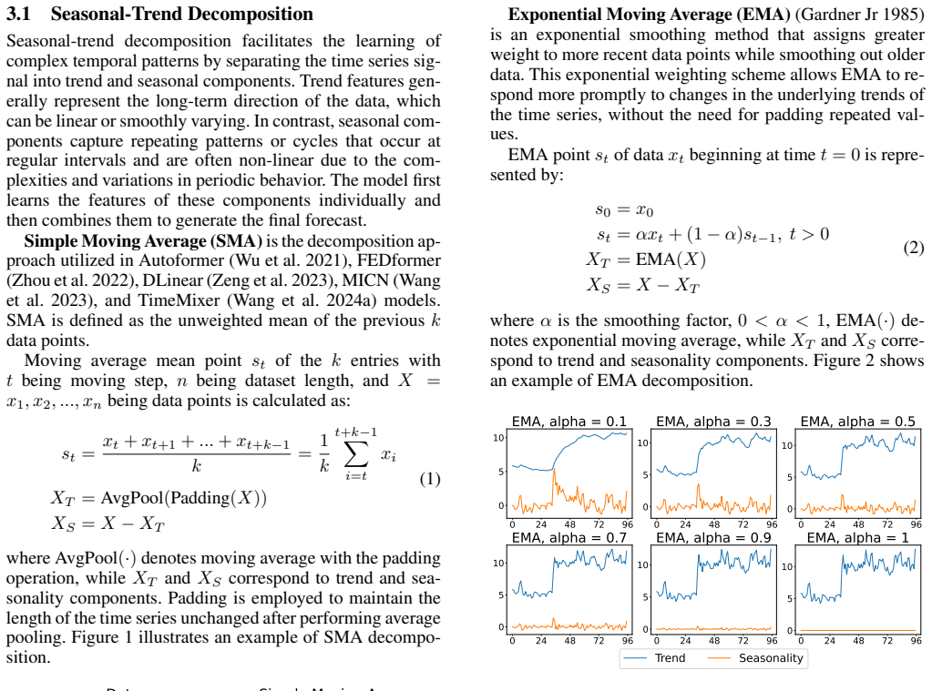
The central object is the exponential seasonal-trend decomposition: with smoothing factor $\alpha$, the trend is $s_t = \alpha x_t + (1-\alpha) s_{t-1}$ and the seasonal component is the residual $x_t - s_t$, computed in $O(1)$ time as a dot product with geometric weights. This replaces the simple moving average decomposition used by several prior models; the trend is sent through a linear MLP stream, while the seasonality is sent through a CNN stream that patches the series into windows of length $P=16$ with stride $S=8$ and applies depthwise separable convolutions with patch-sized kernels. The arctangent loss, with scaling coefficient $\rho(i) = -\arctan(i) + \frac{\pi}{4} + 1$, and a two-sigmoid learning-rate schedule are auxiliary mechanisms claimed to stabilize training and improve accuracy.

What would settle it

Run xPatch and each main baseline (at least CARD, PatchTST, TimeMixer, and iTransformer) in a single codebase on the same GPU, using the same data splits, lookback lengths, prediction horizons, seed protocol, and number of epochs, and check whether the reported margins of roughly 2-8% in MSE and MAE persist; if the margins shrink below noise or reverse, the empirical superiority claim fails.

Watch

Extended reading notes

Core claim

xPatch claims to be the top-performing forecaster among ten compared models on standard long-term forecasting benchmarks, averaged over four prediction horizons, under both a fixed unified protocol and a hyperparameter-search protocol. The empirical anchor is the averaged tables: in unified settings it wins best MSE on 60% of datasets and best MAE on 70%; against CARD it improves by 2.46% in MSE and 2.34% in MAE, and against PatchTST by 4.76% in MSE and 6.20% in MAE. The improvement is attributed to decomposing each univariate series with exponential moving average into trend and seasonal parts, routing them through separate linear and non-linear streams, and training with a robust arctangent loss and a sigmoid learning-rate schedule.

Load-bearing premise

The reported improvements assume that baseline numbers taken from other papers and code repositories were produced under the same experimental conditions as the authors' own runs, including the same history length, training epochs, randomness, data splits, and hardware.

Editorial extensions

If this is right

If the averaged-table results hold, patching and channel independence transfer cleanly from transformer backbones to CNN backbones, so attention is not required to obtain their forecasting benefits.
The EMA decomposition module can replace the simple moving average decomposition in existing models; the paper reports consistent gains on Autoformer, FEDformer, DLinear, and PatchTST.
The arctangent loss and sigmoid learning-rate schedule improve several existing forecasters when used in place of their default training objectives, making these components separable contributions.
xPatch's measured per-step training and inference times are about 3.1 ms and 1.3 ms, several times lower than CARD and TimeMixer, implying comparable accuracy at lower compute if the baseline comparison holds.

Reading between the lines

Editorial extensions of the paper, not claims the author makes directly.

If the baseline-comparability caveat is resolved, the result strengthens the case that permutation-invariant attention is a structural disadvantage for long continuous sequences, since a CNN/MLP model using the same patching and channel-independence recipe matches or beats transformers.
A natural testable extension is to make the smoothing factor $\alpha$ learnable per channel or per dataset; the paper fixes $\alpha = 0.3$ for dual-stream models and $\alpha = 0.1$ for transformer decomposition blocks, suggesting the optimal smoothing level is data-dependent.
The arctangent loss can be viewed as a smooth interpolation between MAE and CARD's signal-decay loss, so it may also benefit other regression tasks with long prediction horizons, which the paper does not explore.
The paper's fair-protocol table shows narrower margins against additional baselines, so a public benchmark that re-runs every method in one environment would settle how much of the reported advantage is architectural rather than protocol-driven.

Share X Bluesky LinkedIn Reddit HN

Editorial analysis

A structured set of objections, weighed in public.

Desk editor's note, referee report, and a circularity audit.

Desk Editor's Note

read the letter

Short version: this is a solid empirical paper, but the headline “better than CARD/PatchTST” claim is not as robust as the writing implies. The architecture is a known dual-stream linear/nonlinear recipe with an EMA-based decomposition module swapped in for the usual SMA, plus patching and channel independence borrowed from PatchTST. What is actually new is narrow: the specific combination, the arctangent loss, and the sigmoid LR schedule. The paper earns credit for being honest about the ablations — EMA on other models, loss and LR comparisons, RevIN effects, and a fair-protocol table without the drop-last trick — and the code is public. The EMA decomposition itself is a genuinely nice tweak: it handles spiky traffic data more sensibly than SMA, and the ADF stationarity analysis in Appendix C is a good check.

Now the soft spots, in proportion to how much they matter. The central empirical claim of SOTA-level superiority depends on baseline numbers that were not produced under the authors' own pipeline. Appendix K says DLinear, TimesNet, ETSformer, FEDformer, and Autoformer results come from the TimesNet repository, and CARD, TimeMixer, iTransformer, and MICN come from their official papers; only RLinear and PatchTST were actually reproduced by the authors. Yet Section 4 says all implementations are derived from official code. That is a real inconsistency. The margins over CARD are 2.46% MSE under unified settings and 5.29% under hyperparameter search, but on Traffic, Electricity, and Exchange, xPatch is actually worse than CARD. The paper reports averages over three seeds but gives no error bars, so we cannot tell whether the 2% gains are noise. The RevIN ablation shows xPatch improves 8.67% with RevIN — larger than the entire claimed margin over CARD — which means any protocol mismatch in how baselines were trained or normalized could flip the ranking. The TFB fair-protocol table (Table 15) partially mitigates this, since baselines there come from a standardized repository, but those baselines are still quoted, not rerun under the exact xPatch evaluation loop.

That said, the core message survives the baseline-comparability critique: a non-transformer with patching and channel independence can be competitive with transformer-based models on standard benchmarks at lower inference cost. That is a useful and mostly credible result for the applied forecasting community, even if the exact ordering against CARD is provisional. The paper deserves a serious referee. I would send it out, with the explicit request that the authors provide seed-wise variance and either rerun the key baselines (at least CARD, PatchTST, TimeMixer) in their own pipeline or clearly mark which numbers are quoted and justify comparability. The architecture and ablations are worth keeping; the SOTA wording needs to be tempered to “competitive on many datasets, not uniformly better.”

Referee Report

4 major / 5 minor

Summary. xPatch is a non-transformer architecture for long-term time series forecasting that decomposes each univariate series via a fixed exponential moving average filter into trend and seasonal components, processes the trend with an MLP stream and the seasonality with a patched depthwise-separable CNN stream, and combines them with a final linear layer. Training uses an arctangent-scaled MAE loss and a sigmoid learning-rate schedule. The paper reports experiments on nine datasets under three protocols (unified lookback, per-model hyperparameter search, and a no-drop-last 'fair' protocol) and compares against eleven baselines, claiming state-of-the-art-level accuracy with lower cost than transformer competitors. Extensive ablations in Appendices E-H and J examine the contribution of each component.

Significance. If the reported results are reproducible and the baselines are genuinely obtained under comparable protocols, xPatch is a meaningful contribution: it shows that patching and channel-independence, previously highlighted in transformer models (PatchTST, CARD), transfer to a strictly convolutional/MLP architecture, and it provides broad ablations with public code. The claimed 2-8% improvements over CARD, TimeMixer, and PatchTST would make xPatch a competitive non-transformer baseline. However, the significance is conditional on baseline comparability and statistical reliability, which are not fully established in this version.

major comments (4)

[§4 and Appendix K] Section 4 states that 'All implementations are derived from the models' official repository code, maintaining the same configurations,' but Appendix K says that DLinear, TimesNet, ETSformer, FEDformer, and Autoformer results are collected from the TimesNet official repository, and CARD, TimeMixer, iTransformer, and MICN results are collected from their respective official papers; only RLinear and PatchTST were reproduced by the authors. These statements conflict for the quoted baselines. Because the headline claim of superiority over CARD (2.46% MSE, Table 13) depends on numbers not produced under the authors' pipeline, and because Appendix J shows that RevIN alone changes xPatch MSE by 8.67%, a small protocol mismatch (lookback length, training epochs, data splits, or normalization) could erase or invert the reported margins. The authors should either rerun all baselines under an identical protocol, or restrict all 'surpasses' claims to rerun baselines and clearly label quoted results as non-comparable.
[Tables 13-15] All main tables report averages over three random seeds but no standard deviations, per-seed values, or significance tests. Many of the reported advantages are within a few percent (e.g., Table 13 ETTh1: xPatch MSE 0.428 vs TimeMixer 0.447; Table 14 ETTm1: 0.341 vs 0.350), and in some settings xPatch is worse than the same baselines (e.g., Table 13 Traffic and Electricity MSE vs CARD, Exchange vs MICN, Solar vs TimeMixer). Without variance information it is impossible to assess whether the claimed improvements exceed seed noise. Please add error bars or per-seed results for the central comparisons.
[Table 15 and Appendix K] The 'fair' protocol without the drop-last trick (Table 15) is the most convincing setup, but it does not include CARD, the main competitor in the headline claim, and its baselines are quoted from the TFB repository rather than rerun in the authors' environment. Thus the comparison with CARD is only shown under the two less-controlled protocols, which is exactly where protocol mismatch is most likely. For the SOTA claim to stand, the fair protocol should include reruns of at least CARD, TimeMixer, and PatchTST under the authors' exact data split, lookback search, and evaluation code.
[§4 (Results) and Table 13] The statement that xPatch 'surpasses CARD by 2.46% in MSE' is based on an average of per-dataset relative differences, computed as 100*(CARD - xPatch)/CARD per dataset and then averaged. This aggregate is dominated by ILI (24.7%) and ETTh2 (13.3%), while xPatch is worse than CARD on four of the ten datasets (Traffic, Electricity, Exchange, Solar). Reporting this single number without per-dataset breakdowns or a significance measure overstates the consistency of the advantage. Please either report the distribution of per-dataset differences or use a more informative summary (e.g., median relative improvement, win/tie/loss counts against each competitor).

minor comments (5)

[Appendix D] The claim that the EMA decomposition module was 'optimized ... to O(1) time complexity' is incorrect: the dot product in Eq. (28) is O(L) for a window of length L. What is achieved is a vectorized computation with precomputed weights, not constant time.
[§3.1, Eq. (1)] The SMA definition writes 'st = (xt+...+xt+k-1)/k' but then defines XT = AvgPool(Padding(X)) without showing the padding operation in the equation; please clarify which side is padded, with what values, and how st relates to the pooled output.
[Table 7, ETTm1, T=192, DLinear* row] The MAE value 0.287 for DLinear* at horizon 192 appears implausibly low compared to the value 0.389 for the original DLinear and is inconsistent with the other horizons in the same block; please check whether this is a typo.
[Appendix J, Table 12 caption] The caption states the comparison is 'between the baselines and the models with RevIN instance normalization,' while the text says the comparison is 'between the original state-of-the-art models and versions trained without using RevIN'; please make the direction and the meaning of the asterisk unambiguous.
[Table 6] The notation 'S (max 25) ↓' is unclear; please define what the downward arrow and 'S' refer to (presumably the number of stationary chunks) and explain the table's reading order.

Circularity Check

0 steps flagged · score 1.0 of 10

No load-bearing circularity: the EMA decomposition, dual-stream forecast, arctangent loss, and sigmoid schedule are evaluated on held-out splits; the flagged issues (quoted baselines, promised-but-omitted proofs, benchmark-informed hyperparameters) are reproducibility risks, not circular derivations.

full rationale

xPatch's derivation chain is self-contained, and I found no step that reduces to its own inputs by construction. The EMA decomposition (Eq. 2) is a fixed transform given alpha: X_T = EMA(X), X_S = X - X_T, which is an additive identity reconstructing X from its components; neither component is defined in terms of the forecasting target. The final prediction (Eq. 12) is a trained linear combination of the MLP stream (Eqs. 3-4) and the CNN stream (Eqs. 5-11), with weights learned against held-out ground truth, and all headline results (Tables 1, 2, 13, 14) are test-set evaluations on separate splits, not fits renamed as predictions. The arctangent loss (Eqs. 16-17) and sigmoid learning-rate schedule (Eq. 23) are training schemes tested in controlled ablations (Tables 8-11); their hyperparameters (alpha = 0.3, m = 1, k = 0.5, s = 10, w = 10, P = 16, S = 8) are chosen by ablation rather than per-dataset test-set fitting, which is mild selection bias typical of the field, not a self-definitional reduction. There are no load-bearing self-citations: the reference list contains no works by the present authors, and the external anchors (Gardner Jr 1985 for exponential smoothing; CARD (Wang et al. 2024b) for the scalable MAE loss family) are independent sources. Two issues are flagged but are correctness risks, not circularity. First, Section 4 states 'All implementations are derived from the models' official repository code, maintaining the same configurations,' while Appendix K states that 'Baseline results for DLinear, TimesNet, ETSformer, FEDformer, and Autoformer are collected from the TimesNet official repository' and 'Results for CARD, TimeMixer, iTransformer, and MICN, which were implemented under the same experimental settings, are collected from their respective official papers'; because most baselines were not rerun under the xPatch pipeline, the claimed 2.46% MSE margin over CARD rests on cross-paper protocol comparability, and Table 15 (TFB protocol) only partially mitigates this. Second, Appendices G and H promise 'Mathematical proofs' of the two training schemes, but only ablation tables appear; the proofs are omitted. Neither issue makes any prediction equivalent to its input by construction, so the honest circularity finding is a low score near zero.

Assumptions & free parameters 5 free parameters · 5 assumptions · 0 invented entities

The central claim is empirical: a specific architecture with tuned hyperparameters outperforms baselines. The main parameters are selected via ablations on the same benchmarks; the evaluation assumes baseline numbers from official papers are comparable. No invented entities or postulates beyond standard ML components are introduced.

free parameters (5)

EMA smoothing factor alpha = 0.3
Chosen after ablation on Weather, Traffic, Electricity (Appendix E); fixed across datasets, not learned.
Arctangent loss scaling m = 1
Ablation found no benefit from scaling (Table 8, Appendix G); m=1 is the unscaled function.
Sigmoid LR hyperparameters (k, s, w) = k=0.5, s=10, w=10
Selected from grid search in Table 10 (Appendix H).
Patch length P and stride S = P=16, S=8
Adopted from PatchTST/CARD for fair comparison; not tuned.
Lookback length L = varies per dataset (e.g., 96, 192, 336, 512, 720)
Hyperparameter search picks best L per dataset for xPatch (Appendix I).

assumptions (5)

domain assumption EMA decomposition with alpha=0.3 yields a stationary seasonal component and non-stationary trend, improving forecastability.
Supported by ADF tests in Appendix C, but this is an empirical regularity, not a theorem.
domain assumption A dual-stream architecture (linear MLP for trend, non-linear CNN for seasonality) captures the respective components better than a single stream.
Tested in Appendix F ablation, but not theoretically justified.
domain assumption Channel-independence (treating each variate separately) is beneficial for multivariate LTSF.
Borrowed from DLinear/PatchTST; validated empirically on benchmarks, not universally true.
domain assumption Baseline numbers collected from official papers are directly comparable to numbers produced by the authors.
Used throughout Section 4 and Appendix K; mismatched protocols would invalidate the comparison.
standard math Standard mathematical definitions of EMA, convolution, pooling, normalization.
Background math used without proof.

how reviews work

0 comments

Cite this review

Pith. "Pith review of xPatch: Dual-Stream Time Series Forecasting with Exponential Seasonal-Trend Decomposition." pith.science (2026). https://pith.science/paper/V4SZFYHK

@misc{pith2026241217323,
  author       = {Pith},
  title        = {Pith review of: xPatch: Dual-Stream Time Series Forecasting with Exponential Seasonal-Trend Decomposition},
  year         = {2026},
  howpublished = {\url{https://pith.science/paper/V4SZFYHK}},
  note         = {Machine review of arXiv:2412.17323}
}

read the original abstract

In recent years, the application of transformer-based models in time-series forecasting has received significant attention. While often demonstrating promising results, the transformer architecture encounters challenges in fully exploiting the temporal relations within time series data due to its attention mechanism. In this work, we design eXponential Patch (xPatch for short), a novel dual-stream architecture that utilizes exponential decomposition. Inspired by the classical exponential smoothing approaches, xPatch introduces the innovative seasonal-trend exponential decomposition module. Additionally, we propose a dual-flow architecture that consists of an MLP-based linear stream and a CNN-based non-linear stream. This model investigates the benefits of employing patching and channel-independence techniques within a non-transformer model. Finally, we develop a robust arctangent loss function and a sigmoid learning rate adjustment scheme, which prevent overfitting and boost forecasting performance. The code is available at the following repository: https://github.com/stitsyuk/xPatch.

Figures

Figures reproduced from arXiv: 2412.17323 by the authors.

**Figure 2.** Example of EMA decomposition with α = {0.1, 0.3, 0.5, 0.7, 0.9, 1} on a 96-length sample from the ETTh1 dataset. The exponential method offers greater control over the behavior of both trend and seasonality components. Given that data can exhibit diverse patterns, including stationary and non-stationary characteristics with varying periods and behaviors, the adaptability of exponential decomposition provides adva… view at source ↗

**Figure 1.** Example of SMA decomposition with kernel k = [PITH_FULL_IMAGE:figures/full_fig_p003_1.png] view at source ↗

**Figure 3.** xPatch Model Overview. Every univariate series is passed through exponential decomposition. Consequently, the [PITH_FULL_IMAGE:figures/full_fig_p004_3.png] view at source ↗

Figures from the paper (18 more)

**Figure 4.** Figure 4: SMA and EMA smoothing and decomposition on [PITH_FULL_IMAGE:figures/full_fig_p010_4.png]

**Figure 5.** Figure 5: Forecasting performance (MAE), lookback win [PITH_FULL_IMAGE:figures/full_fig_p012_5.png]

**Figure 6.** Figure 6: Separate forecasting performance (MAE) of [PITH_FULL_IMAGE:figures/full_fig_p013_6.png]

**Figure 7.** Figure 7: Comparison between the arctangent function and [PITH_FULL_IMAGE:figures/full_fig_p013_7.png]

**Figure 9.** Figure 9: LTSF learning rate adjustment strategies. [PITH_FULL_IMAGE:figures/full_fig_p015_9.png]

**Figure 8.** Figure 8: Sigmoid function with different (k, s, w) parame [PITH_FULL_IMAGE:figures/full_fig_p015_8.png]

**Figure 11.** Figure 11: Sample prediction graph of the next T = 96 points with lookback window L = 336 from the ETTh1 dataset. [PITH_FULL_IMAGE:figures/full_fig_p021_11.png]

**Figure 12.** Figure 12: Sample prediction graph of the next T = 192 points with lookback window L = 96 from the ETTh2 dataset. [PITH_FULL_IMAGE:figures/full_fig_p021_12.png]

**Figure 13.** Figure 13: Sample prediction graph of the next T = 336 points with lookback window L = 96 from the ETTh2 dataset. [PITH_FULL_IMAGE:figures/full_fig_p022_13.png]

**Figure 14.** Figure 14: Sample prediction graph of the next T = 720 points with lookback window L = 96 from the ETTm2 dataset. [PITH_FULL_IMAGE:figures/full_fig_p022_14.png]

**Figure 15.** Figure 15: Sample prediction graph of the next T = 96 points with lookback window L = 96 from the Electricity dataset. [PITH_FULL_IMAGE:figures/full_fig_p023_15.png]

**Figure 16.** Figure 16: Sample prediction graph of the next T = 60 points with lookback window L = 36 from the Illness dataset. [PITH_FULL_IMAGE:figures/full_fig_p023_16.png]

**Figure 17.** Figure 17: Sample prediction graph of the next T = 192 points with lookback window L = 96 from the ETTh2 dataset. [PITH_FULL_IMAGE:figures/full_fig_p024_17.png]

**Figure 18.** Figure 18: Sample prediction graph of the next T = 96 points with lookback window L = 96 from the Electricity dataset. [PITH_FULL_IMAGE:figures/full_fig_p024_18.png]

**Figure 19.** Figure 19: Sample prediction graph of the next T = 48 points with lookback window L = 36 from the Illness dataset. [PITH_FULL_IMAGE:figures/full_fig_p024_19.png]

**Figure 20.** Figure 20: Sample prediction graph of the next T = 96 points with lookback window L = 96 from the Weather dataset. [PITH_FULL_IMAGE:figures/full_fig_p025_20.png]

**Figure 21.** Figure 21: Sample prediction graph of the next T = 192 points with lookback window L = 96 from the Weather dataset. [PITH_FULL_IMAGE:figures/full_fig_p025_21.png]

**Figure 22.** Figure 22: Sample prediction graph of the next T = 336 points with lookback window L = 96 from the Weather dataset. [PITH_FULL_IMAGE:figures/full_fig_p025_22.png]

Discussion (0). Continue with ORCID to comment.

Reference graph

Works this paper leans on

32 extracted references · 5 canonical work pages

[1]

, " * write output.state after.block = add.period write newline

ENTRY address archivePrefix author booktitle chapter edition editor eid eprint howpublished institution isbn journal key month note number organization pages publisher school series title type volume year label extra.label sort.label short.list INTEGERS output.state before.all mid.sentence after.sentence after.block FUNCTION init.state.consts #0 'before.a...
[2]

write newline

" write newline "" before.all 'output.state := FUNCTION n.dashify 't := "" t empty not t #1 #1 substring "-" = t #1 #2 substring "--" = not "--" * t #2 global.max substring 't := t #1 #1 substring "-" = "-" * t #2 global.max substring 't := while if t #1 #1 substring * t #2 global.max substring 't := if while FUNCTION word.in bbl.in capitalize " " * FUNCT...
[3]

Bahdanau, D.; Cho, K.; and Bengio, Y. 2015. Neural machine translation by jointly learning to align and translate. In International Conference on Learning Representations

work page 2015
[4]

E.; Jenkins, G

Box, G. E.; Jenkins, G. M.; Reinsel, G. C.; and Ljung, G. M. 2015. Time series analysis: forecasting and control. John Wiley & Sons

2015
[5]

A.; and Fuller, W

Dickey, D. A.; and Fuller, W. A. 1979. Distribution of the estimators for autoregressive time series with a unit root. Journal of the American statistical association, 74(366a): 427--431

work page 1979
[6]

Dosovitskiy, A.; Beyer, L.; Kolesnikov, A.; Weissenborn, D.; Zhai, X.; Unterthiner, T.; Dehghani, M.; Minderer, M.; Heigold, G.; Gelly, S.; Uszkoreit, J.; and Houlsby, N. 2021. An Image is Worth 16x16 Words: Transformers for Image Recognition at Scale. ICLR

2021
[7]

Gardner Jr, E. S. 1985. Exponential smoothing: The state of the art. Journal of forecasting, 4(1): 1--28

work page 1985
[8]

Han, L.; Ye, H.-J.; and Zhan, D.-C. 2023. The Capacity and Robustness Trade-off: Revisiting the Channel Independent Strategy for Multivariate Time Series Forecasting. arXiv preprint arXiv:2304.05206

arXiv 2023

Show all 32 references

[9]

Hendrycks, D.; and Gimpel, K. 2016. Gaussian error linear units (gelus). arXiv preprint arXiv:1606.08415

2016 arXiv
[10]

G.; Zhu, M.; Chen, B.; Kalenichenko, D.; Wang, W.; Weyand, T.; Andreetto, M.; and Adam, H

Howard, A. G.; Zhu, M.; Chen, B.; Kalenichenko, D.; Wang, W.; Weyand, T.; Andreetto, M.; and Adam, H. 2017. Mobilenets: Efficient convolutional neural networks for mobile vision applications. arXiv preprint arXiv:1704.04861

2017 arXiv
[11]

Ioffe, S.; and Szegedy, C. 2015. Batch normalization: Accelerating deep network training by reducing internal covariate shift. In International conference on machine learning, 448--456. pmlr

2015
[12]

Kim, T.; Kim, J.; Tae, Y.; Park, C.; Choi, J.-H.; and Choo, J. 2021. Reversible instance normalization for accurate time-series forecasting against distribution shift. In International Conference on Learning Representations

2021
[13]

Lai, G.; Chang, W.-C.; Yang, Y.; and Liu, H. 2018. Modeling long-and short-term temporal patterns with deep neural networks. In The 41st international ACM SIGIR conference on research & development in information retrieval, 95--104

2018
[14]

Li, S.; Jin, X.; Xuan, Y.; Zhou, X.; Chen, W.; Wang, Y.-X.; and Yan, X. 2019. Enhancing the locality and breaking the memory bottleneck of transformer on time series forecasting. Advances in neural information processing systems, 32

2019
[15]

Li, Z.; Qi, S.; Li, Y.; and Xu, Z. 2023. Revisiting Long-term Time Series Forecasting: An Investigation on Linear Mapping. arXiv preprint arXiv:2305.10721

2023 arXiv
[16]

Liu, Y.; Hu, T.; Zhang, H.; Wu, H.; Wang, S.; Ma, L.; and Long, M. 2024. iTransformer: Inverted Transformers Are Effective for Time Series Forecasting. In The Twelfth International Conference on Learning Representations

2024
[17]

Liu, Y.; Wu, H.; Wang, J.; and Long, M. 2022. Non-stationary transformers: Exploring the stationarity in time series forecasting. Advances in Neural Information Processing Systems, 35: 9881--9893

2022
[18]

Nguyen, N.; Sinthong, P.; and Kalagnanam, J

Nie, Y.; H. Nguyen, N.; Sinthong, P.; and Kalagnanam, J. 2023. A Time Series is Worth 64 Words: Long-term Forecasting with Transformers. In International Conference on Learning Representations

2023
[19]

Paszke, A.; Gross, S.; Massa, F.; Lerer, A.; Bradbury, J.; Chanan, G.; Killeen, T.; Lin, Z.; Gimelshein, N.; Antiga, L.; et al. 2019. Pytorch: An imperative style, high-performance deep learning library. Advances in neural information processing systems, 32

2019
[20]

Trockman, A.; and Kolter, J. Z. 2022. Patches Are All You Need? Trans. Mach. Learn. Res

2022
[21]

N.; Kaiser, .; and Polosukhin, I

Vaswani, A.; Shazeer, N.; Parmar, N.; Uszkoreit, J.; Jones, L.; Gomez, A. N.; Kaiser, .; and Polosukhin, I. 2017. Attention is all you need. Advances in neural information processing systems, 30

2017
[22]

Wang, H.; Peng, J.; Huang, F.; Wang, J.; Chen, J.; and Xiao, Y. 2023. Micn: Multi-scale local and global context modeling for long-term series forecasting. In The eleventh international conference on learning representations

2023
[23]

Y.; and Zhou, J

Wang, S.; Wu, H.; Shi, X.; Hu, T.; Luo, H.; Ma, L.; Zhang, J. Y.; and Zhou, J. 2024 a . Timemixer: Decomposable multiscale mixing for time series forecasting. arXiv preprint arXiv:2405.14616

2024 arXiv
[24]

Wang, X.; Zhou, T.; Wen, Q.; Gao, J.; Ding, B.; and Jin, R. 2024 b . CARD : Channel Aligned Robust Blend Transformer for Time Series Forecasting. In The Twelfth International Conference on Learning Representations

2024
[25]

Wen, Q.; Zhou, T.; Zhang, C.; Chen, W.; Ma, Z.; Yan, J.; and Sun, L. 2022. Transformers in time series: A survey. arXiv preprint arXiv:2202.07125

2022 arXiv
[26]

Woo, G.; Liu, C.; Sahoo, D.; Kumar, A.; and Hoi, S. 2022. Etsformer: Exponential smoothing transformers for time-series forecasting. arXiv preprint arXiv:2202.01381

2022 arXiv
[27]

Wu, H.; Hu, T.; Liu, Y.; Zhou, H.; Wang, J.; and Long, M. 2023. TimesNet: Temporal 2D-Variation Modeling for General Time Series Analysis. In International Conference on Learning Representations

2023
[28]

Wu, H.; Xu, J.; Wang, J.; and Long, M. 2021. Autoformer: Decomposition transformers with auto-correlation for long-term series forecasting. Advances in Neural Information Processing Systems, 34: 22419--22430

2021
[29]

Zeng, A.; Chen, M.; Zhang, L.; and Xu, Q. 2023. Are transformers effective for time series forecasting? In Proceedings of the AAAI conference on artificial intelligence, volume 37, 11121--11128

2023
[30]

Zhang, Y.; and Yan, J. 2022. Crossformer: Transformer utilizing cross-dimension dependency for multivariate time series forecasting. In The Eleventh International Conference on Learning Representations

2022
[31]

Zhou, H.; Zhang, S.; Peng, J.; Zhang, S.; Li, J.; Xiong, H.; and Zhang, W. 2021. Informer: Beyond efficient transformer for long sequence time-series forecasting. In Proceedings of the AAAI conference on artificial intelligence, volume 35, 11106--11115

2021
[32]

Zhou, T.; Ma, Z.; Wen, Q.; Wang, X.; Sun, L.; and Jin, R. 2022. Fedformer: Frequency enhanced decomposed transformer for long-term series forecasting. In International Conference on Machine Learning, 27268--27286. PMLR

2022

Pith tools

Reviewed August 11, 2026 · model on record in the stance chip above.

[1] [1]

, " * write output.state after.block = add.period write newline

ENTRY address archivePrefix author booktitle chapter edition editor eid eprint howpublished institution isbn journal key month note number organization pages publisher school series title type volume year label extra.label sort.label short.list INTEGERS output.state before.all mid.sentence after.sentence after.block FUNCTION init.state.consts #0 'before.a...

[2] [2]

write newline

" write newline "" before.all 'output.state := FUNCTION n.dashify 't := "" t empty not t #1 #1 substring "-" = t #1 #2 substring "--" = not "--" * t #2 global.max substring 't := t #1 #1 substring "-" = "-" * t #2 global.max substring 't := while if t #1 #1 substring * t #2 global.max substring 't := if while FUNCTION word.in bbl.in capitalize " " * FUNCT...

[3] [3]

Bahdanau, D.; Cho, K.; and Bengio, Y. 2015. Neural machine translation by jointly learning to align and translate. In International Conference on Learning Representations

work page 2015

[4] [4]

E.; Jenkins, G

Box, G. E.; Jenkins, G. M.; Reinsel, G. C.; and Ljung, G. M. 2015. Time series analysis: forecasting and control. John Wiley & Sons

2015

[5] [5]

A.; and Fuller, W

Dickey, D. A.; and Fuller, W. A. 1979. Distribution of the estimators for autoregressive time series with a unit root. Journal of the American statistical association, 74(366a): 427--431

work page 1979

[6] [6]

Dosovitskiy, A.; Beyer, L.; Kolesnikov, A.; Weissenborn, D.; Zhai, X.; Unterthiner, T.; Dehghani, M.; Minderer, M.; Heigold, G.; Gelly, S.; Uszkoreit, J.; and Houlsby, N. 2021. An Image is Worth 16x16 Words: Transformers for Image Recognition at Scale. ICLR

2021

[7] [7]

Gardner Jr, E. S. 1985. Exponential smoothing: The state of the art. Journal of forecasting, 4(1): 1--28

work page 1985

[8] [8]

Han, L.; Ye, H.-J.; and Zhan, D.-C. 2023. The Capacity and Robustness Trade-off: Revisiting the Channel Independent Strategy for Multivariate Time Series Forecasting. arXiv preprint arXiv:2304.05206

arXiv 2023