REVIEW 4 major objections 5 minor 17 references
Explaining Data Mixing Scaling Laws
T0 review · 4 major / 5 minor · reviewed 2026-08-02 · deepseek-v4-flash
Pith's one-line read A model's loss on a mixed-domain dataset reduces to two mechanisms: capacity competition between skills and noise reduction from seeing a domain's own tokens.
desk verdict A genuinely new two-term data-mixing law with a real out-of-sample cross-scale test, but the formal derivation rests on an unsupported (and numerically wrong) constancy assumption for the noise coefficient. read the letter →
The pith
A machine-rendered reading of the paper's core claim, the machinery that carries it, and where it could break.
The reading
What carries the argument
The central object is the two-term loss identity L_i ≈ c_i x_i^{-b_i} + A_i(Dh_i)^{-a_i} + E_i, together with the capacity-allocation problem that defines x_i^*. The entire derivation rides on the 'shared head, disjoint tail' spectral structure: domains share a common set of top eigenvectors, and each domain's exclusive tail eigenvalues decay as k^{-α_i}. Under that structure, a projected linear regression trained by one-pass SGD can be analyzed in closed form, with the approximation error matching the capacity term and the variance error matching the noise term.
What would settle it
Vary label noise in one domain across several levels, train small models on a fixed set of mixtures, fit the two-term law, and check whether the fitted A_i for each domain is stable across mixtures with different Σ h_j σ_j². If A_i shifts systematically with h (e.g., with the proportion of the noisy domain), the constant-A assumption is falsified. A second falsifier: compute the predicted optimal mixture for two scales with the same fitted parameters and compare with empirically evaluated mixtures at both scales; a mismatch in the direction or magnitude of the shift would falsify the scale-ext
Extended reading notes
Core claim
Under the 'shared head, disjoint tail' spectral assumption, the expected test loss on domain i satisfies L_i(h,N,D) ≈ c_i x_i^*(h,N)^{-b_i} + A_i(Dh_i)^{-a_i} + E_i, where x_i^*(h,N) is the optimal capacity allocation from the convex program min Σ h_j c_j x_j^{-b_j} subject to Σ(x_j−H) ≤ N−H. The first term comes from the mass of unlearned specialized skills and couples all domains through the shadow price of capacity; the second term is the variance error of one-pass SGD and is inversely proportional to the number of tokens seen from that domain. The decomposition explains the empirically observed domain interaction and, critically, predicts that the optimal mixture shifts as model size and
Load-bearing premise
Everything rests on the assertion that the noise coefficient A(h) — which the formal theorem shows depends on the mixture-weighted sum of per-domain label variances — is close enough to a constant that the fitted form A_i(Dh_i)^{-a_i} is faithful; if per-domain label noise differs strongly, A(h) varies with h and the derived loss law is not the one the theorem proves.
Editorial extensions
If this is right
- If the two-term decomposition holds, practitioners can fit its ~5K parameters on small proxy runs and solve the convex inner problem to predict the optimal mixture for much larger models and token budgets, without retraining.
- The noise term A_i(Dh_i)^{-a_i} explains why optimal mixtures over-weight hard-to-learn domains: the term decays fastest for domains with small h_i, pushing the optimum toward larger weights for high-A_i, low-α_i domains.
- Because the capacity term couples all domains through the Lagrange multiplier, the framework predicts that the loss landscape is not separable: changing the weight of one domain shifts all domain losses, a coupling that empirical exponential laws cannot represent.
- The framework predicts a specific scale-dependence of the optimal mixture: as D grows, the noise term shrinks, so the optimal mixture moves toward the capacity-only optimum, which the authors show can be below or above the target weights depending on domain exponents.
Reading between the lines
- A direct stress test of the framework would vary label noise across domains: because the formal theorem's A(h) contains Σ h_j σ_j², the constant-A assumption should fail when label noise is strongly heterogeneous. If the fitted A_i then varies systematically with h, the derived functional form is not the one the theorem establishes.
- The shared-head/disjoint-tail assumption suggests a natural perturbation theory: for domains with moderate tail overlap, one would expect a correction term that is small but grows with overlap; the paper's own synthetic experiments suggest the model is robust up to ~40% intersection, so a next step is to derive the first-order correction in overlap.
- The capacity-allocation problem's convexity in a transformed variable could be exploited to replace the current non-convex fitting with a convex relaxation, making parameter estimation more reliable and cheaper.
- The framework's focus on in-distribution domain loss leaves open how to adapt it to downstream tasks or unseen domains; the same two-term logic might hold but with the capacity term replaced by a task-specific skill-importance vector.
Editorial analysis
A structured set of objections, weighed in public.
Referee Report
Summary. The paper proposes a unified theoretical framework for multi-domain data-mixing scaling laws. It assumes a 'shared head, disjoint tail' spectral/skill structure across domains and argues that the loss on domain i for a model trained on mixture h is governed by two mechanisms: capacity competition, modeled through a convex capacity-allocation program whose solution x_i^*(h,N) yields a c_i x_i^*(h,N)^{-b_i} term, and noise reduction, modeled through a per-domain term A_i(D h_i)^{-a_i}. The main claimed result, Theorem 4.1 (formalized as Theorem D.19), states this two-term decomposition up to asymptotic relative error. The paper fits the constants on small-scale runs and uses the resulting law to predict held-out mixtures, optimal mixtures, and mixtures at larger unseen scales, reporting lower MRE than empirical baselines and competitive extrapolation performance on Pile and SlimPajama.
Significance. If the derivation were sound, this would be a valuable first-principles account of data-mixing scaling laws, with the notable strength of using far fewer free parameters than existing empirical laws and being validated by genuine cross-scale extrapolation. The appendix contains a substantial asymptotic analysis, and the empirical protocol is a reasonable out-of-sample test. However, two load-bearing technical issues prevent the paper from establishing its central claim as stated: the formal theorem's noise coefficient is mixture-dependent and is treated as a per-domain constant via an unsupported assumption, and the variance analysis only covers a narrower exponent range than the theorem asserts. The empirical results are promising but do not, by themselves, resolve these theoretical gaps.
major comments (4)
- [Section D.8, Assumption D.18; Theorem D.19; Eq. (3)] The formal theorem D.19 gives the loss term A(h)/(D h_tau)^{1-1/alpha_tau}, where A(h) = Gamma(1-1/alpha_tau)/(alpha_tau(2 eta_0)^{1-1/alpha_tau}) + (sum_i h_i sigma_i^2) C_{alpha_tau} I_gamma eta_0^{1/alpha_tau}. This coefficient depends on h whenever the per-domain label noises sigma_i^2 differ, but Eq. (3) and Theorem 4.1 use per-domain constants A_i. Assumption D.18 asserts A(h) ≈ constant and claims numerical support A(h)∈[8,9] for alpha∈[1,3], eta∈[0.1,1], sigma_i^2≤1. That numerical claim is incorrect: for alpha=1.5, eta=0.1 the first term alone is about 3.1, and for alpha=2, eta=1 it is about 0.63, so the bracketing is not valid. More fundamentally, no evidence is given that the h-dependent second term is negligible for the actual Pile/SlimPajama domains. If it is not negligible, the fitted A_i absorb an h-dependent quantity, and the functional form used for the bi-level optimum,
- [Section D.7, Lemma D.15 vs Assumption D.4; Theorem D.13] Lemma D.15 explicitly assumes 1 < alpha < 2 and defines I_gamma = ∫_0^1 [1+cos G(pi(1-v))] v^{1/alpha-2} dv as a finite constant. For alpha >= 2, the exponent 1/alpha - 2 <= -3/2, so the integral diverges. Assumption D.4 allows alpha_i in [1,3], and Theorem D.19 states the result for all such alpha. Thus the variance bounds used in Theorem D.13 and the final theorem do not cover the declared parameter range. The proof of Theorem D.19 also relies on 1/3 - 1/alpha_tau > 0, which fails at alpha_tau = 3. The theorem's scope must be restricted to alpha < 2, or the variance analysis must be extended to larger alpha.
- [Section 4.3, Eq. (4); Assumption D.1; Section 5.2, fitting procedure] The formal theorem and all variance/bias bounds require Assumption D.1, i.e. h_i >= h > 0 for all i. The optimal-mixture problem in Eq. (4), however, is solved over the closed simplex, and the fitting procedure in Section 5.2 explicitly discards data with h_i = 0 because of the (N h_i)^{-a} term. The predicted optimal mixture h* could therefore lie on the boundary, outside the regime where the asymptotic expansion is proved. The paper should either extend the analysis to boundary points with suitable limiting arguments or discuss and test whether the predicted optima are interior.
- [Figure 4 and Section 5.4] The paper claims in the 7-domain 1B/30B extrapolation that the proposed law 'achieves the same final test loss' as the full-data baseline. The reported final losses are 2.1087 and 2.1106, a difference of about 0.002, which is very likely within training noise for single runs. No error bars, multiple seeds, or statistical test are reported. This overstates the strength of the cross-scale comparison. The result is still suggestive, but the claim of matching the baseline should be tempered or supported by variance estimates.
minor comments (5)
- [Section D.8] In the proof/statement of Theorem D.19, 'With Theorem D.18' should read 'With Assumption D.18'; D.18 is an assumption, not a theorem.
- [Theorem D.19 statement] The formal statement omits Assumption D.6, although the proof uses it to control terms like D^{-2(1+epsilon)(1-1/alpha_tau)}. The assumption should be included in the theorem statement.
- [Table 2 and Eq. (1)] The parameter counts for 'Ours (Eq. (1))' and 'Ours (Eq. 3)' appear to omit the shared-head boundary H. If H is a fitted parameter, the counts should be 3K+1 and 5K+1; if H is fixed, this should be stated.
- [Figure 1] The synthetic stress test for tail overlap lacks details on the generative process, the number of trials, and how the overlap parameter p is implemented. Without this, the robustness claim in Section 4.1 is hard to evaluate.
- [Captions and references] Figure 2 and Figure 3 captions cite 'Shukor et al., 2025' while the reference list gives 2026; please harmonize. Also, Eq. (3) should state explicitly that a_i = 1 - 1/alpha_i, matching Theorem D.19.
Circularity Check
No significant circularity: cross-scale predictions are out-of-sample; the main weakness (Assumption D.18's constant A(h)) is a rigor/robustness concern, not a self-referential reduction.
full rationale
The paper's central empirical claim is cross-scale extrapolation, and that test is genuinely out-of-sample: Section 5.4 fits the Extended Linear Regression Model parameters exclusively on small-scale losses (122M/10B) and then substitutes the target (N,D)=(1B,30B) into the fitted law to solve for an extrapolated mixture; the strong baseline, by contrast, is fitted on a range of scales that explicitly includes the target 1B/30B losses. Thus the headline comparison does not reduce to fitting the target quantity. The theoretical chain is also a real derivation rather than a tautology: Theorem D.9 proves that the approximation error of the top-N sketched linear regression is equal, up to a discretization gap, to the Extended Quantization Model's capacity-allocation loss; Theorems D.12 and D.13 evaluate the bias and variance terms; Theorem D.19 combines them into the two-term loss bound. The loss is not defined as Eq. 3; it is computed from the sketched linear model under explicit spectral assumptions. The main caveat is Assumption D.18, which replaces the formally mixture-dependent noise coefficient A(h) with a constant A, and supports this with a bracketing claim (A(h)∈[8,9]) that appears numerically suspect. If A(h) is not actually constant on real Pile/SlimPajama mixtures, the fitted A_i will absorb h-dependent variation and the fitted functional form will not be exactly the form established by Theorem D.19. This is an important correctness and robustness issue, but it is not circular: the empirical constants are fitted, target-scale losses are not used in fitting the proposed law, and no fitted parameter is renamed as a prediction. There is also no load-bearing self-citation chain: the cited theoretical frameworks (Lin et al., Bordelon et al., Li et al., Pan et al.) are external prior work. Overall, the derivation is self-contained against the key out-of-sample benchmark, so the circularity score is low.
Assumptions & free parameters
free parameters (6)
- c_i (per-domain capacity loss scale) =
fitted
- b_i = α_i - 1 (per-domain tail exponent) =
fitted
- E_i (per-domain irreducible loss) =
fitted
- A_i (per-domain noise amplitude) =
fitted
- a_i (per-domain noise exponent) =
fitted
- H (shared-head boundary) =
unspecified
assumptions (11)
- domain assumption Power-law frequency/eigenvalue spectrum within each domain (λ_k^(i) = k^{-α_i}, α_i > 1)
- domain assumption Shared head, disjoint tail: all domain covariance matrices are simultaneously diagonalizable, and tail eigenvectors of different domains are orthogonal
- ad hoc to paper Assumption D.1: every domain weight h_i ≥ h > 0
- domain assumption Assumption D.2: hypercontractivity of domain distributions
- domain assumption Assumption D.3: isotropic teacher prior E[θ* θ*^⊤] = I
- domain assumption Assumption D.4: 1 < α_i ≤ 3
- domain assumption Assumption D.5: training loss is bounded above
- domain assumption Assumption D.6: N^{α_i} ≥ D^{1+ε}
- ad hoc to paper Assumption D.18: A(h) = Γ(1-1/α_τ)/(α_τ(2η0)^{1-1/α_τ}) + (Σ_i h_i σ_i²) C Iγ η0^{1/α_τ} ≈ constant A
- domain assumption The overlapping/shared-head loss is nearly constant when mixture weights change
- standard math SDE approximation of one-pass SGD with cosine LR and Itô calculus
Cite this review
Pith. "Pith review of Explaining Data Mixing Scaling Laws." pith.science (2026). https://pith.science/paper/VR7643PR
@misc{pith2026260608167,
  author       = {Pith},
  title        = {Pith review of: Explaining Data Mixing Scaling Laws},
  year         = {2026},
  howpublished = {\url{https://pith.science/paper/VR7643PR}},
  note         = {Machine review of arXiv:2606.08167}
}
read the original abstract
Recent research has established empirical scaling laws to predict model performance on multi-domain data mixtures. However, a theoretical understanding of these model loss behaviors remains absent. In this work, we propose a unified framework to explain the underlying mechanics of data mixing. Our approach extends theoretical perspectives originally developed for standard neural scaling laws (e.g., Kaplan and Chinchilla) to the multi-domain setting. Based on the distributional assumption that domains overlap on fundamental skills while diverging on specialized skills, we identify two key factors that govern the domain losses of models trained on different data mixtures: \textit{Capacity Competition}, where the allocation of finite model capacity couples domain losses globally, and \textit{Noise Reduction}, where optimal weights shift toward harder-to-learn domains to minimize overall noise. Empirical evaluations show that our framework outperforms existing baselines by fitting the loss landscape with a lower Mean Relative Error and identifying higher-performing training mixtures. Most importantly, our model successfully extrapolates across scales, predicting highly effective mixtures for large, unseen scales using parameters fitted on smaller ones. In addition, our model achieves these results using significantly fewer parameters compared to previous empirical laws. Our code is available at https://github.com/meiqwq/Explaining-Data-Mixing-Scaling-Laws.
Figures

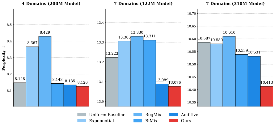

Figures from the paper (2 more)


Reference graph
Works this paper leans on
-
[1]
Albalak, A., Pan, L., Raffel, C., and Wang, W. Y. Efficient online data mixing for language model pre-training. arXiv preprint arXiv:2312.02406,
-
[3]
Atanasov, A., Zavatone-Veth, J. A., and Pehlevan, C. Scaling and renormalization in high-dimensional regression.arXiv preprint arXiv:2405.00592,
-
[4]
resolves
Table 4: Hyperparameters for the 200M and 700M proxy models used in our data mixing experiments. Hyperparameter 200M Model 700M Model Architecture Layers (L) 24 24 Hidden Size (d model) 768 1536 Attention Heads 12 12 Sequence Length 1024 1024 Optimization Global Batch Size 128 128 Micro Batch Size 16 16 Learning Rate 3.5×10 −4 3.5×10 −4 Minimum Learning R...
2024
-
[7]
The pile: An 800gb dataset of diverse text for language modeling.arXiv preprint arXiv:2101.00027,
Gao, L., Biderman, S., Black, S., Golding, L., Hoppe, T., Foster, C., Phang, J., He, H., Thite, A., Nabeshima, N., et al. The pile: An 800gb dataset of diverse text for language modeling.arXiv preprint arXiv:2101.00027,
-
[8]
16 Gu, X., Lyu, K., Li, J., and Zhang, J
URLhttps://openreview.net/forum?id=JsM46OZix7. 16 Gu, X., Lyu, K., Li, J., and Zhang, J. Data mixing can induce phase transitions in knowledge acquisition. In ICLR 2025 Workshop on Navigating and Addressing Data Problems for Foundation Models,
2025
-
[9]
Hoffmann, J., Borgeaud, S., Mensch, A., Buchatskaya, E., Cai, T., Rutherford, E., Casas, D
URL https://openreview.net/forum?id=ZKA4yiGdrA. Hoffmann, J., Borgeaud, S., Mensch, A., Buchatskaya, E., Cai, T., Rutherford, E., Casas, D. d. L., Hendricks, L. A., Welbl, J., Clark, A., et al. Training compute-optimal large language models.arXiv preprint arXiv:2203.15556,
-
[10]
Kaplan, J., McCandlish, S., Henighan, T., Brown, T
URL https: //openreview.net/forum?id=rujwIvjooA. Kaplan, J., McCandlish, S., Henighan, T., Brown, T. B., Chess, B., Child, R., Gray, S., Radford, A., Wu, J., and Amodei, D. Scaling laws for neural language models.arXiv preprint arXiv:2001.08361,
arXiv 2001
-
[12]
URL https://openreview.net/forum?id=p9YlQPF8fE. Maloney, A., Roberts, D. A., and Sully, J. A solvable model of neural scaling laws.arXiv preprint arXiv:2210.16859,
Show all 17 references
-
[13]
Zhang, P., Zeng, G., Wang, T., and Lu, W
URL https://openreview.net/forum?id=kJ5i29FejW. Zhang, P., Zeng, G., Wang, T., and Lu, W. Tinyllama: An open-source small language model.arXiv preprint arXiv:2401.02385,
-
[14]
18 A Empirical Data Mixing Laws As detailed in Table 3, these baselines offer distinct functional forms for predicting the domain loss Li(h) given the data mixture weights h. Specifically, we consider: (1) theAdditive Law(Shukor et al., 2026), which models the loss using an in...
2026
-
[15]
19 C Implementation Details For the experiments in Section 5.3, we implement our pretraining pipeline using the Megatron-LM framework in Korthikanti et al
12:end while 13:Return:Optimal mixtureh ∗ ←h (t). 19 C Implementation Details For the experiments in Section 5.3, we implement our pretraining pipeline using the Megatron-LM framework in Korthikanti et al. (2022) on a cluster of 8 NVIDIA H200 GPUs. To investigate the scaling l...
2022
-
[17]
In the following section, λk denotes the eigenvalue associated with the eigenvector uk, i.e.H uk = λkuk (but not the k-th largest eigenvalue)
+ i. In the following section, λk denotes the eigenvalue associated with the eigenvector uk, i.e.H uk = λkuk (but not the k-th largest eigenvalue). In this basis with flattened index,A i is diagonal withA i = diag(a1, a2, . . .) and ak =u ⊤ k Aiuk = ( l−αi k= Γ(i, l) 0 otherwi...
2020
-
[1987]
URL https: //opg.optica.org/josaa/abstract.cfm?URI=josaa-4-12-2379
doi: 10.1364/JOSAA.4.002379. URL https: //opg.optica.org/josaa/abstract.cfm?URI=josaa-4-12-2379. Fonseca, N., Lee, S. H., Mingard, C., Louis, A., et al. An exactly solvable model for emergence and scaling laws in the multitask sparse parity problem.Advances in Neural Informati...
-
[2022]
Li, B., Chen, F., Huang, Z., Wang, L., and Wu, L
URL https://arxiv.org/abs/2205.05198. Li, B., Chen, F., Huang, Z., Wang, L., and Wu, L. Functional scaling laws in kernel regression: Loss dynamics and learning rate schedules. InThe Thirty-ninth Annual Conference on Neural Information Processing Systems, 2026a. URLhttps://ope...
-
[2023]
and Goyal, A
Arora, S. and Goyal, A. A theory for emergence of complex skills in language models.arXiv preprint arXiv:2307.15936,
-
[2024]
URL https://www.pnas.org/doi/abs/10.1073/pnas.2311878121
doi: 10.1073/pnas.2311878121. URL https://www.pnas.org/doi/abs/10.1073/pnas.2311878121. Bordelon, B., Atanasov, A., and Pehlevan, C. A dynamical model of neural scaling laws. InInternational Conference on Machine Learning, pp. 4345–4382. PMLR,
-
[2025]
Brown, T., Mann, B., Ryder, N., Subbiah, M., Kaplan, J
URL https://openreview.net/ forum?id=dEypApI1MZ. Brown, T., Mann, B., Ryder, N., Subbiah, M., Kaplan, J. D., Dhariwal, P., Neelakantan, A., Shyam, P., Sastry, G., Askell, A., et al. Language models are few-shot learners.Advances in neural information processing systems, 33:1877–1901,
1901
Reviewed August 2, 2026 · model on record in the stance chip above.
Discussion (0). Continue with ORCID to comment.