Kinetic closure of turbulence: collision-side modeling beyond the filtered BGK--Boltzmann equation
Pith reviewed 2026-05-20 02:06 UTC · model grok-4.3
The pith
Filtering the Boltzmann equation concentrates turbulence closure on modeling non-Markovian collisions from subgrid residuals.
A machine-rendered reading of the paper's core claim, the machinery that carries it, and where it could break.
Core claim
In the dilute-gas LES and RANS regimes the main limitation of Boltzmann and BGK-type collision models is not the breakdown of molecular chaos but the retention of a Markovian collision process at a scale where filtering induces finite temporal correlations in the collision product. The closure problem is therefore dual: one must infer the filtered fine-grained equilibrium, which is not computable from filtered moments alone, and model the non-Markovian collision dynamics generated by the collision-product covariance. The framework makes this dual structure explicit and represents the resulting collision-covariance source term through a BGK-like closure built from the subgrid equilibrium残差, 湍
What carries the argument
The dual closure problem of inferring the filtered fine-grained equilibrium and modeling non-Markovian collision dynamics from collision-product covariance, represented by a BGK-like closure on the subgrid equilibrium residual with a phenomenological turbulent relaxation frequency.
If this is right
- The Chapman-Enskog analysis follows the kinetic-to-macroscopic timescale ratio that arises from nondimensionalization and avoids artificial turbulent scale separations.
- Higher moments retain an additional Mach dependence through the mixed scaling of particle velocity.
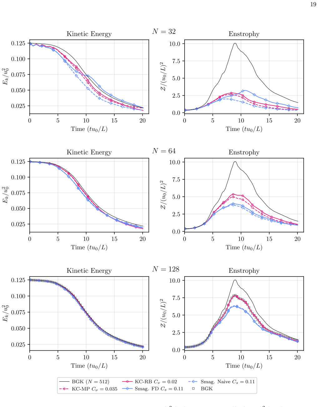
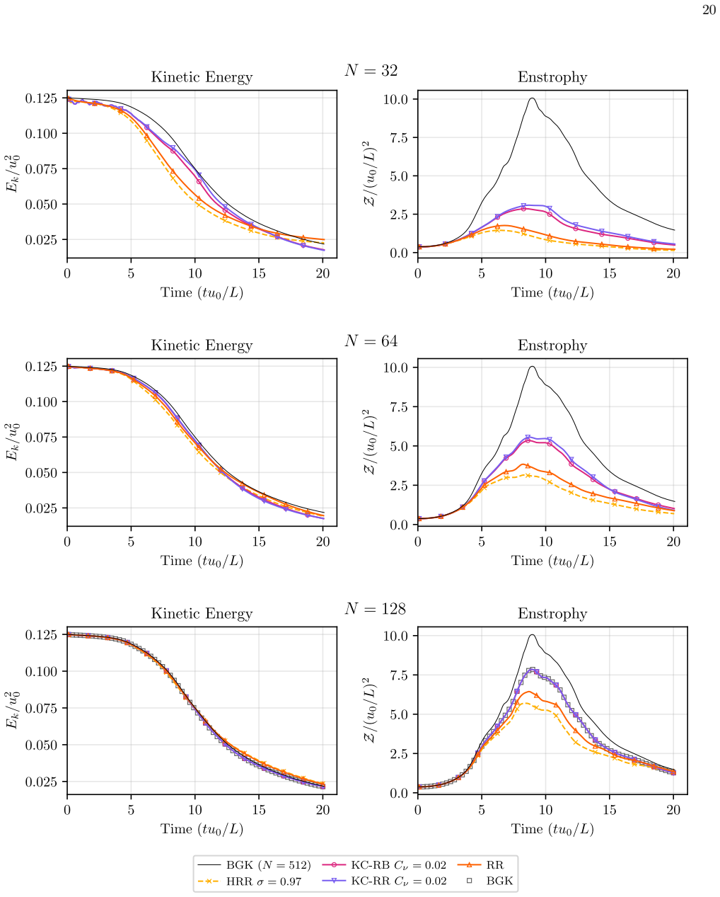
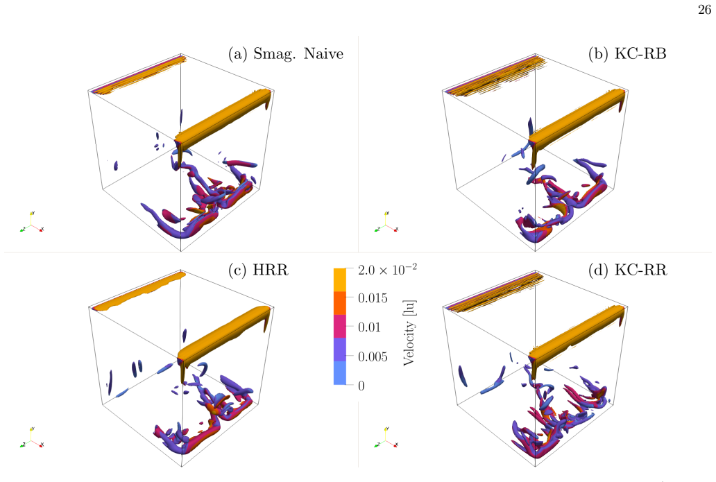
- The closures can be implemented in lattice Boltzmann simulations and compared directly with the Smagorinsky model and regularization-based collision models.
Where Pith is reading between the lines
- The same dual-structure perspective could be used to construct closures for other filtered kinetic equations that retain a streaming operator.
- Replacing the phenomenological relaxation frequency with a derived expression would allow the model to be applied across wider ranges of Reynolds and Mach numbers without additional tuning.
- The approach suggests a route to consistent subgrid modeling in lattice Boltzmann methods that remains inside the kinetic description rather than reverting to macroscopic eddy-viscosity forms.
Load-bearing premise
That a first phenomenological realization of the turbulent relaxation frequency suffices to capture the non-Markovian collision dynamics without derivation from first principles or external benchmarks.
What would settle it
A high-resolution simulation or measurement that extracts the collision-product covariance directly in a filtered turbulent flow and compares it quantitatively against the value predicted by the proposed BGK-like closure.
Figures


read the original abstract
This article extends a recently introduced kinetic closure of turbulence by developing its theoretical framework, operational realizations, and validation. In contrast with filtered Navier--Stokes formulations, filtering the Boltzmann equation retains subgrid advective transport under the linear streaming operator, so that unresolved physics is concentrated on the collision side. We show that in the dilute-gas LES and RANS regimes, the main limitation of Boltzmann and BGK-type collision models is not the breakdown of molecular chaos, but the retention of a Markovian collision process at a scale where filtering induces finite temporal correlations in the collision product. In a BGK-type framework, the closure problem is dual: one must infer the filtered fine-grained equilibrium, which is not computable from filtered moments alone, and model the non-Markovian collision dynamics generated by the collision-product covariance. The present framework makes this dual structure explicit and represents the resulting collision-covariance source term through a BGK-like closure built from the subgrid equilibrium residual, with the turbulent relaxation frequency given by a first phenomenological realization. The framework relies on a Chapman--Enskog analysis organized by the reference timescale ratio emerging directly from the nondimensionalization of the kinetic equation and performed in the classical sense, thereby avoiding artificial turbulent scale separations. We show that the Chapman--Enskog structure is not a pure one-parameter Knudsen scaling: the primary ordering is set by the kinetic-to-macroscopic timescale ratio, while higher moments retain an additional Mach dependence through the mixed scaling of particle velocity. The resulting kinetic closures are validated through lattice Boltzmann simulations and compared with the Smagorinsky model and regularization-based collision models.
Editorial analysis
A structured set of objections, weighed in public.
Referee Report
Summary. The manuscript extends a kinetic closure for turbulence by shifting focus to the collision side of the filtered BGK-Boltzmann equation. It frames the closure problem as dual—inferring the filtered fine-grained equilibrium (not recoverable from filtered moments alone) and modeling non-Markovian collision dynamics arising from collision-product covariance—and closes the resulting source term with a BGK-like operator constructed from the subgrid equilibrium residual. The turbulent relaxation frequency is supplied by a first phenomenological realization. A Chapman–Enskog expansion is performed using the kinetic-to-macroscopic timescale ratio obtained directly from nondimensionalization (with additional Mach dependence retained in higher moments), and the resulting closures are stated to be validated via lattice Boltzmann simulations against the Smagorinsky model and regularization-based alternatives.
Significance. If the phenomenological frequency can be shown to be robust across flows and if quantitative validation confirms that the dual closure improves subgrid transport predictions without ad-hoc tuning, the work would provide a distinct route to subgrid modeling in kinetic LES/RANS that preserves advective subgrid contributions under the streaming operator. The explicit separation of equilibrium inference from collision covariance modeling is a conceptual strength, but the current reliance on a single tunable element limits immediate applicability.
major comments (3)
- [Abstract] Abstract: the claim of validation through lattice Boltzmann simulations supplies no quantitative results, error metrics, or comparison tables; without these, it is impossible to evaluate whether the collision-covariance closure improves upon the Smagorinsky or regularization baselines.
- [Framework description] Framework description (abstract and subsequent sections introducing the closure): the turbulent relaxation frequency is introduced solely as a 'first phenomenological realization' without derivation from first principles, moment-matching constraints, or external benchmark data. Because this frequency directly supplies the BGK-like term that closes the collision-product covariance, any mismatch propagates into the retained subgrid advective transport and the Chapman–Enskog ordering.
- [Chapman–Enskog analysis] Chapman–Enskog analysis section: the expansion is organized exclusively by the kinetic-to-macroscopic timescale ratio from nondimensionalization, without additional external calibration or moment constraints that would fix the relaxation frequency independently of the target flow; this leaves the ordering dependent on the same phenomenological element used for closure.
minor comments (2)
- Notation for the subgrid equilibrium residual should be defined explicitly at first use and distinguished from the filtered equilibrium to avoid ambiguity in the dual-closure discussion.
- The manuscript would benefit from a brief statement of the specific functional form chosen for the phenomenological relaxation frequency, even if only illustrative.
Simulated Author's Rebuttal
We thank the referee for the constructive and detailed comments. We address each major comment point by point below, indicating planned revisions where appropriate.
read point-by-point responses
-
Referee: [Abstract] Abstract: the claim of validation through lattice Boltzmann simulations supplies no quantitative results, error metrics, or comparison tables; without these, it is impossible to evaluate whether the collision-covariance closure improves upon the Smagorinsky or regularization baselines.
Authors: We agree that the abstract lacks quantitative indicators. In the revised manuscript we will add concise statements of key error metrics and performance comparisons drawn from the lattice Boltzmann results already reported in the body of the paper. The full tables, figures, and quantitative comparisons against Smagorinsky and regularization-based models remain in the results section. revision: yes
-
Referee: [Framework description] Framework description (abstract and subsequent sections introducing the closure): the turbulent relaxation frequency is introduced solely as a 'first phenomenological realization' without derivation from first principles, moment-matching constraints, or external benchmark data. Because this frequency directly supplies the BGK-like term that closes the collision-product covariance, any mismatch propagates into the retained subgrid advective transport and the Chapman–Enskog ordering.
Authors: The manuscript deliberately presents the frequency as a first phenomenological realization because the primary contribution is the explicit dual-closure structure (equilibrium inference plus collision-covariance modeling) rather than a universal derivation of the frequency itself. We acknowledge that this choice limits immediate robustness across flows, as noted in the referee’s significance assessment. We will insert a short clarifying paragraph in the framework section stating the phenomenological status and indicating that future calibration against moment constraints or benchmark data is planned. revision: partial
-
Referee: [Chapman–Enskog analysis] Chapman–Enskog analysis section: the expansion is organized exclusively by the kinetic-to-macroscopic timescale ratio from nondimensionalization, without additional external calibration or moment constraints that would fix the relaxation frequency independently of the target flow; this leaves the ordering dependent on the same phenomenological element used for closure.
Authors: The expansion is organized by the timescale ratio that emerges directly from nondimensionalization precisely to avoid introducing artificial turbulent scale separations. The retained Mach dependence in higher moments follows from the mixed scaling of particle velocity and is already stated in the manuscript. Because the frequency remains phenomenological, its influence on the ordering is intrinsic to the present realization. We will expand the discussion in the Chapman–Enskog section to make this dependence and its implications for the closure more explicit. revision: partial
Circularity Check
No significant circularity; derivation grounded in nondimensionalization and explicit phenomenological assumption
full rationale
The paper's central construction explicitly introduces the turbulent relaxation frequency as a first phenomenological realization within a BGK-like closure for the collision-covariance term, rather than deriving it by construction from filtered moments or prior fitted quantities. The Chapman-Enskog analysis is organized directly from the kinetic-to-macroscopic timescale ratio obtained via nondimensionalization of the kinetic equation, using classical ordering without artificial scale separations or self-referential reductions. No load-bearing step equates a claimed prediction or first-principles result to its own inputs; the dual closure structure is made explicit as an extension of standard kinetic theory, with the phenomenological element stated as an assumption rather than a self-defining or fitted-output quantity. Self-citation to prior work on the kinetic closure is present but not load-bearing for the current derivations.
Axiom & Free-Parameter Ledger
free parameters (1)
- turbulent relaxation frequency
axioms (1)
- domain assumption Chapman-Enskog analysis organized by reference timescale ratio from nondimensionalization of the kinetic equation, performed in the classical sense
invented entities (1)
-
subgrid equilibrium residual
no independent evidence
Lean theorems connected to this paper
-
IndisputableMonolith/Cost/FunctionalEquation.leanwashburn_uniqueness_aczel unclear?
unclearRelation between the paper passage and the cited Recognition theorem.
the closure problem is dual: one must infer the filtered fine-grained equilibrium... and model the non-Markovian collision dynamics generated by the collision-product covariance... with the turbulent relaxation frequency given by a first phenomenological realization
-
IndisputableMonolith/Foundation/RealityFromDistinction.leanreality_from_one_distinction unclear?
unclearRelation between the paper passage and the cited Recognition theorem.
Chapman–Enskog analysis organized by the reference timescale ratio emerging directly from the nondimensionalization... ϵ ≡ Ma²/Re_ℓ = τ_mft/T
What do these tags mean?
- matches
- The paper's claim is directly supported by a theorem in the formal canon.
- supports
- The theorem supports part of the paper's argument, but the paper may add assumptions or extra steps.
- extends
- The paper goes beyond the formal theorem; the theorem is a base layer rather than the whole result.
- uses
- The paper appears to rely on the theorem as machinery.
- contradicts
- The paper's claim conflicts with a theorem or certificate in the canon.
- unclear
- Pith found a possible connection, but the passage is too broad, indirect, or ambiguous to say the theorem truly supports the claim.
Reference graph
Works this paper leans on
-
[1]
The Gibbs ensemble average⟨·⟩ens, representing an expectation over realizations of initial microscopic configurations
-
[2]
The macroscopic temporal average⟨·⟩∆t, evaluated over a finite time window∆t within a single realiza- tion. The one-particle distribution functionF corresponds directly to the ensemble average of the exact field: F(z,t) =⟨N(z,t)⟩ens.(A3) The ensemble-averaged product of the field decomposes as [11, 83] ⟨N(z,t)N(zii,t)⟩ens =F 2(z,zii,t) +δ(z−zii)F(z,t), (A...
-
[3]
Collision-side-only scaling in a filtered formulation The filtered formulation of [25] states that the hydro- dynamic limit of the filtered Boltzmann equation reads (Eq. (41) in [25]): 0 =∂t˜u♭ α1 +∂α1 ( ¯p♭ ¯ρ ) +∂α2 ( ˜u♭ α1 ˜u♭ α2 ) −2Kn∂(1) α2 ˜S♭ α1α2 + Kn 12∂α3 [ ( ˜S♭ α1α3−W♭ α1α3)( ˜S♭ α3α2 +W♭ α3α2) ] , (B1) with the resolved strain and rotation ...
-
[4]
The equa- tion employs the molecularKn as the sole pertur- bation parameter
Incorrect asymptotic Ma scaling. The equa- tion employs the molecularKn as the sole pertur- bation parameter. In the present convective scal- ing, however, the CE expansion is controlled by the timescale ratio ϵ=τmft/(L/U) = MaKn supplied by the nondimensionalization. In [25], Ma∼1, so Kn∼1/Re, and the stress corrections multiplied by Kn in Eq. (B1) are v...
-
[5]
Incorrect placement of the SGS stress. The leading O(1)terms in Eq. (B1) form an unfiltered Euler or a filtered-laminar Euler system, so the mo- mentum flux contains no SGS contribution. In LES, the filtered Euler equations contain theO(1)SGS stress tensormsgs α1α2 because inertial energy transfer enters through the advective flux. By placing the non-line...
-
[6]
Approximate Deconvolution Method Consider the BE for the unfiltered distributionf: ∂tf+ξα∂αf=Q(f).(B8) In the ADM formulation [27, 28], a deconvolved distri- bution f∗is introduced to approximate the unfiltered state, with the reconstruction errorf′≡f−f∗. Thisf′ is functionally analogous to the SGS carrierfsgs of the present work: both represent the devia...
-
[7]
targets a different representation: it rewrites the moment-level advective commutation structure into ex- plicit transformed transport and acceleration terms by changing variables to a moving velocity frame. This ap- pendix analyzes what that representation changes in the filtered hierarchy, first at Euler level and then in the modeled kinetic equation us...
-
[8]
Herex♭andξ♭are the convectively nondimensional spatial and velocity coordinates
Non-orthogonality of relative phase-space coordinates In the standard kinetic description, the one-particle phase space is the product of physical space and velocity space,Γ = x♭×ξ♭. Herex♭andξ♭are the convectively nondimensional spatial and velocity coordinates. The coordinate directions are defined by the partial derivatives e♭ xα≡∂♭ α ⏐⏐ ξ♭,e ♭ ξβ≡∂♭ ξ...
-
[9]
The relative-frame BGK equation When rewriting the inertial streaming operator in the moving, non-inertial coordinates, the chain rule generates explicitlyη♭-dependent transport terms, including a force- like velocity-space derivative. Applying the filter operator over the transformed variables yields the following relative- 36 frame kinetic equation repo...
-
[10]
(45) the SGS stress appears at leading order through the second raw moment off(0) =f(0) +fsgs
Euler limit In the inertial-frame Euler limit already derived in Eq. (45) the SGS stress appears at leading order through the second raw moment off(0) =f(0) +fsgs. In contrast, the Euler level component of Eq. (C10) reads ∂(1) t g(0) +η♭ α1∂(1) α1g(0)−∂♭ ηα2 (g(0)A♭(1) α2 ) =ω♯g(1).(C11) This equation shows the effect of Girimaji’s closure at Euler order....
-
[11]
(C12) Thus, the unresolved covariancemsgs α1α2 is absent from this equilibrium contribution
Relative streaming flux:Under this assumed equilib- rium closure, the second moment of the relative equi- librium, m(0) α1α2 = ∫ η♭ α1η♭ α2g(0)dη♭, contains only the resolved advective part and the thermal pressure: m(0) α1α2 = ∫ η♭ α1η♭ α2g(0)dη♭ = ¯ρ˜u♭ α1 ˜u♭ α2 + ¯p♭δα1α2. (C12) Thus, the unresolved covariancemsgs α1α2 is absent from this equilibrium ...
-
[12]
Force-like moment:The acceleration termA♭ α2 con- tributes through the velocity-space derivative. Inte- gration by parts gives − ∫ η♭ α1∂♭ ηα2 ( g(0)A♭(1) α2 ) dη♭= ∫ g(0)A♭(1) α1 dη♭,(C13) where A♭(1) α2 ≡∂(1) t u′♭ α2 +η♭ α3∂(1) α3u′♭ α2 +u′♭ α3∂(1) α3u′♭ α2 denotes the induced phase-space acceleration at the convective scale. Under the same incompressi...
-
[13]
A CE expansion could in principle be car- ried out in the relative variables by using Eq
Navier–Stokes-order limit The work [29] does not perform a CE but only a change of variables. A CE expansion could in principle be car- ried out in the relative variables by using Eq. (C11) to express g(1) in theO(ϵ2)equation to see the effect of the collision-relaxation in the relative reference frame (rhs of Eq. (C9)). Equation (C11) shows that the tran...
-
[14]
LES stress model With the notation used here and without the CE-order decomposition, the closed equation actually advanced in
-
[15]
(19) of [29] corresponds to ∂♭ tg+η♭ α1∂♭ α1g−¯ρ−1∂♭ α2msgs α1α2∂♭ ηα1 g=−ϵω♯(g−g(0))
uses (gu′♭α1)≈0,(C15) (gA♭α1)≈g¯ρ−1∂♭ α2msgs α1α2.(C16) Thus Eq. (19) of [29] corresponds to ∂♭ tg+η♭ α1∂♭ α1g−¯ρ−1∂♭ α2msgs α1α2∂♭ ηα1 g=−ϵω♯(g−g(0)). (C17) In [29], msgs α1α2 is not computed from the relative-frame kinetic equation but is prescribed by a Smagorinsky SGS model
-
[16]
Conclusions The relative-frame transformation does not remove the SGS influence from the kinetic dissipative problem; it rewrites the transport-side contribution while leaving the collision-side closure unaddressed. At Euler level it recov- ers the same unclosed second-order stress content already carried byfsgs in the inertial filtered formulation, but r...
-
[17]
Top-down projection of the Navier–Stokes equations Chen’s approach [43] defines a probability density func- tion ψ(x,ξ,t)for an ensemble of infinitesimal fluid ele- ments. In its incompressible form, this PDF is normalized as ∫ ψdξ= 1, so its moments give the hydrodynamic veloc- ity directly rather than density-weighted kinetic moments. The evolution ofψo...
-
[18]
Averaging and the emergence of the collision term We denote the average used in [43] with a local space– time filtering notation, δψ≡ψ−ψ, δAα≡Aα−Aα. (D4) Chen et al. describe this operation as an ensemble average of fluid elements. In the present comparison, however, ⟨·⟩ens denotes the molecular ensemble average that defines the one-particle distributionF...
-
[19]
(D12) constrains the second moment ofC, but it does not determine the full collision operator
The difference in closure strategy The energy identity Eq. (D12) constrains the second moment ofC, but it does not determine the full collision operator. The closure adopted in [43, 44] then assumes that the covariance-driven interaction relaxesψtoward a Gaussian target. The target is centered atuαto preserve momentum. Its width is set by a reduced equili...
-
[20]
Summary Chen’s approach and the present one [3] both go be- yond the simple calculation of fine-grained equilibrium or the modeling of the advective SGS term, and instead focus on modeling unresolved covariance-driven kinetic source terms. However, the two frameworks diverge at the closure level, as summarized in Table V: Chen’s Klimon- tovichformulationi...
-
[21]
At each fluid node and before collision (after streaming):
Common operational algorithm The operational update used in the simulations follows the standard collide–stream sequence. At each fluid node and before collision (after streaming):
-
[22]
compute the local macroscopic fields from the shifted populations, ¯ρ= ∑ i fi,¯ρ˜u α= ∑ i fiξiα;(F20)
-
[23]
constructthelocalequilibrium f(0) i =f(0) i (¯ρ,˜u)from Eq. (F15)
-
[24]
(F16) and (F17) (or use a weighted lattice- link stencil [86], not tested herein)
evaluate the velocity gradients and Sα1α2 from Eqs. (F16) and (F17) (or use a weighted lattice- link stencil [86], not tested herein)
-
[25]
compute the closure-specific SGS tracemsgs α1α1 used below, from Eqs. (F24), (F31) and (F38)
-
[26]
The quantityρ0 is the fixed ref- erence density used by the discrete implementation
evaluate the SGS amplitude and the clipped turbu- lent relaxation frequency through ksgs≈1 2ρ0 ⏐⏐msgs α1α1 ⏐⏐, ρ 0 = 1lu, νeff t = max ( ν,Cν∆ √ ksgs ) , ˆωsgs = (νeff t θR + ∆t 2 )−1 = min ˆω, ( Cν∆ √ ksgs θR + ∆t 2 )−1 ; (F21) Here ksgs, νeff t , and∆are the lattice-unit counter- parts ofk♯ sgs, ν♯ t, and∆ ♯ x, after the clipping by the molecular v...
-
[27]
apply the closure-specific collision rule: Eq. (F25) for KC-RB, Eq. (F34) for KC-MP, and Eqs. (F39), (F42) and (F44) for KC-RR
-
[28]
For the uniform lattices considered here,∆ = ∆x
stream the post-collision populations. For the uniform lattices considered here,∆ = ∆x
-
[29]
Step 4: SGS traceThe SGS trace is obtained as fol- lows:
Operational implementation of KC-RB After the common pre-collision steps of Appendix F1, the model-specific part enters through steps 4 and 6. Step 4: SGS traceThe SGS trace is obtained as fol- lows:
-
[30]
approximate the resolved first-order CE carrier, f(1) i ≈−wi ¯ρˆτ θR Hiα1α2Sα1α2,(F22) where Hiα1α2≡ξiα1ξiα2−θRδα1α2;(F23)
-
[31]
form the SGS residual, fsgs,i≡fi−f(0) i −f(1) i .(F8)
-
[32]
compute the SGS trace used in the turbulent relax- ation model, msgs α1α1 = ∑ i fsgs,iξ2 i ;(F24) Step 6: collision ruleThe post-collision populations are fpost i =fi−∆tˆωf(1) i −∆tˆωsgsfsgs,i;(F25) The simulations reported in the present paper did not use this Hermite-consistent form. To remain aligned with the original incompressible formulation propose...
-
[33]
Step 4: SGS traceThe SGS trace is obtained as fol- lows:
Operational implementation of KC-MP After the common pre-collision steps of Appendix F1, the model-specific part enters through steps 4 and 6. Step 4: SGS traceThe SGS trace is obtained as fol- lows:
-
[34]
approximate the resolved first-order CE stress, m(1) α1α2≈−2¯ρθRˆτSα1α2;(F28)
-
[35]
compute the coarse non-equilibrium stress, mcneq α1α2 = ∑ i (fi−f(0) i )ξiα1ξiα2;(F29)
-
[36]
subtract the resolved part to obtain the SGS stress, msgs α1α2 =m cneq α1α2−m(1) α1α2;(F30)
-
[37]
take the trace used in the turbulent relaxation model, msgs α1α1 =m cneq α1α1−m(1) α1α1.(F31) Step 6: collision ruleThe collision rule is applied as follows:
-
[38]
reconstruct the SGS carrier, fsgs,i = wi 2θ2 R Hiα1α2msgs α1α2;(F32)
-
[39]
identify the operational resolved first-order carrier, f(1) i ≈(fi−f(0) i )−fsgs,i;(F33)
-
[40]
apply the split collision rule, fpost i =fi−∆tˆωf(1) i −∆tˆωsgsfsgs,i;(F34) Because the reconstruction is performed in the same Her- mite basis, no additional compressibility error analogous to the KC-RBξξ-approximation is introduced here
-
[41]
Operational implementation of KC-RR KC-RR operates directly on the discrete Hermite co- efficients offcneq i =fi−f(0) i , using the Hermite basis introduced in Eq. (F23). At second order, the Hermite coefficient coincides with the raw non-equilibrium moment because ∑ i(fi−f(0) i ) = 0; the second-order coefficient is therefore written below in raw-moment ...
-
[42]
build the second-order regularized seed, arr α1α2≡−2¯ρθRˆτSα1α2;(F35)
-
[43]
compute the second-order coarse non-equilibrium Hermite coefficients, acneq α1α2 = ∑ i (fi−f(0) i )ξiα1ξiα2;(F36)
-
[44]
define the SGS second-order coefficients, asgs α1α2 =a cneq α1α2−arr α1α2;(F37)
-
[45]
Thus higher powers are not independent on the lattice
take the trace used in the turbulent relaxation model, msgs α1α1≡asgs α1α1 =a cneq α1α1−arr α1α1.(F38) Step 6: collision ruleFor the higher-order projection, D3Q27 provides only three independent lattice functions in each Cartesian direction:1, ξiα, andξ2 iα−θR. Thus higher powers are not independent on the lattice. For example, ξ3 iα= (∆x/∆t)2ξiα. Conseq...
-
[46]
relax the second-order coefficients, apost xx = (1−∆tˆω)arr xx + (1−∆tˆωsgs)asgs xx, apost yy = (1−∆tˆω)arr yy + (1−∆tˆωsgs)asgs yy, apost zz = (1−∆tˆω)arr zz + (1−∆tˆωsgs)asgs zz , apost xy = (1−∆tˆω)arr xy + (1−∆tˆωsgs)asgs xy, apost xz = (1−∆tˆω)arr xz + (1−∆tˆωsgs)asgs xz, apost yz = (1−∆tˆω)arr yz + (1−∆tˆωsgs)asgs yz ; (F39) 45
-
[47]
compute the high-order D3Q27 Hermite coefficients, acneq α1...αn = ∑ i (fi−f(0) i )Hi,α1...αn,(α 1...αn)∈Bhigh, (F40) where no component inBhigh contains a directional power above two
-
[48]
compute the regularized higher-order coefficients froma rr α1α2 with the RR recursion, arr α1...αn = ˜u♭ αnarr α1...αn−1 + 1 ¯ρ n−1∑ i=1 a(0) α1...αi−1αi+1...αn−1arr αiαn, (82)
-
[49]
define the SGS high-order coefficients, asgs α1...αn =a cneq α1...αn−arr α1...αn,(α 1...αn)∈Bhigh;(F41)
-
[50]
relax the higher-order coefficients, apost α1...αn = (1−∆tˆω)arr α1...αn + (1−∆tˆωsgs)asgs α1...αn,(α 1...αn)∈Bhigh; (F42)
-
[51]
define the directional discrete Hermite factors, Hx,i≡ξix, H xx,i≡ξ2 ix−θR, Hy,i≡ξiy, H yy,i≡ξ2 iy−θR, Hz,i≡ξiz, H zz,i≡ξ2 iz−θR, (F43)
-
[52]
reconstruct the post-collision populations, fpost i =f (0) i +wi 6∑ m=2 Tm,(F44) where T2 = 1 2θ2 R [ Hxx,iapost xx +Hyy,iapost yy +Hzz,iapost zz ] + 1 θ2 R [ Hx,iHy,iapost xy +Hx,iHz,iapost xz +Hy,iHz,iapost yz ] , T3 = 1 2θ3 R [ Hxx,iHy,iapost xxy +Hxx,iHz,iapost xxz +Hyy,iHz,iapost yyz ] + 1 2θ3 R [ Hx,iHyy,iapost xyy +Hx,iHzz,iapost xzz +Hy,iHzz,iapos...
-
[53]
(F7) can be derived directly from the KC-RB split in the transformed equa- tion Eq
Trapezoidal reconstruction of the two-rate collision The explicit two-rate update in Eq. (F7) can be derived directly from the KC-RB split in the transformed equa- tion Eq. (F3), with the local relaxation times held fixed during the collision step. The update is explicit only after expressingQi(f)in terms offi. For clarity, first recall the unshifted rela...
-
[54]
S. B. Pope,Turbulent flows(Cambridge University Press, Cambridge; New York, 2000)
work page 2000
-
[55]
S. Chapman and T. Cowling,The Mathematical Theory of Non-uniform Gases: An Account of the Kinetic Theory of Viscosity, Thermal Conduction and Diffusion in Gases, Cambridge Mathematical Library (Cambridge University Press, 1953)
work page 1953
- [56]
-
[57]
Krieger, Molecular theory of isotropic turbulence, Physics of Fluids4, 649 (1961)
I. Krieger, Molecular theory of isotropic turbulence, Physics of Fluids4, 649 (1961)
work page 1961
-
[58]
V. N. Zhigulev, Equations for the Turbulent Motion of a Gas, Doklady Akademii Nauk SSSR165, 502 (1965)
work page 1965
-
[59]
S. Tsuge, Approach to the origin of turbulence on the basis of two-point kinetic theory, Physics of Fluids17, 22 (1974)
work page 1974
-
[60]
G. Chliamovitch, O. Malaspinas, and B. Chopard, Ki- netic Theory beyond the Stosszahlansatz, Entropy19, 381 (2017), publisher: Multidisciplinary Digital Publishing Institute
work page 2017
-
[61]
G. Chliamovitch and Y. Thorimbert, Turbulence through the spyglass of bilocal kinetics, Entropy20, 539 (2018)
work page 2018
-
[62]
P. L. Bhatnagar, E. P. Gross, and M. Krook, A Model for Collision Processes in Gases. I. Small Amplitude Pro- cesses in Charged and Neutral One-Component Systems, Physical Review94, 511 (1954)
work page 1954
-
[63]
S. Tsuge, On the breakdown of the molecular chaos in the presence of translational nonequilibrium, Physics Letters A36, 249 (1971)
work page 1971
-
[64]
S. Tsuge and K. Sagara, A new hierarchy system on the basis of a master boltzmann equation for microscopic density, Journal of Statistical Physics12, 403 (1975)
work page 1975
-
[65]
G. Chliamovitch, O. Malaspinas, and B. Chopard, A Trun- cation Scheme for the BBGKY2 Equation, Entropy17, 7522 (2015)
work page 2015
-
[66]
N. N. Bogoliubov,Problems of Dynamical Theory in Sta- tistical Physics(Gostekhteoretizdat, Moscow–Leningrad,
-
[67]
in Russian; original title: Problemy dinamicheskoi teorii v statisticheskoi fizike
-
[68]
N. N. Bogoliubov, Problems of a dynamical theory in statistical physics, inStudies in Statistical Mechanics, Vol. 1, edited by J. de Boer and G. E. Uhlenbeck (North- Holland, Amsterdam, 1962) pp. 1–118, english translation of the 1946 Russian monograph
work page 1962
-
[69]
M. Born and H. S. Green, A general kinetic theory of liq- uids. i. the molecular distribution functions, Proceedings of the Royal Society of London. Series A, Mathematical and Physical Sciences188, 10 (1946)
work page 1946
-
[70]
J. G. Kirkwood, The statistical mechanical theory of trans- port processes I. general theory, The Journal of Chemical Physics14, 180 (1946)
work page 1946
-
[71]
J. Yvon,La théorie statistique des fluides et l’équation d’état, Actualités scientifiques et industrielles. Théories mécaniques (hydrodynamique-acoustique) No. 203 (Her- mann & Cie, Paris, 1935)
work page 1935
-
[72]
V. Yakhot and S. A. Orszag, Renormalization group anal- ysis of turbulence. I. Basic theory, Journal of Scientific Computing1, 3 (1986)
work page 1986
-
[73]
V. Yakhot and S. A. Orszag, Renormalization-Group Anal- ysis of Turbulence, Physical Review Letters57, 1722 (1986), publisher: American Physical Society
work page 1986
-
[74]
H. Chen, S. Succi, and S. Orszag, Analysis of subgrid scale turbulence using the Boltzmann Bhatnagar-Gross-Krook kinetic equation, Physical Review E59, R2527 (1999), publisher: American Physical Society
work page 1999
-
[75]
H. Chen, S. Kandasamy, S. Orszag, R. Shock, S. Succi, and V. Yakhot, Extended Boltzmann kinetic equation for turbulent flows, Science (New York, N.Y.)301, 633 (2003)
work page 2003
- [76]
-
[77]
H. Chen, S. A. Orszag, I. Staroselsky, and S. Succi, Ex- panded analogy between Boltzmann kinetic theory of fluids and turbulence, Journal of Fluid Mechanics519, 301 (2004)
work page 2004
-
[78]
O. Malaspinas and P. Sagaut, Consistent subgrid scale modelling for lattice Boltzmann methods, Journal of Fluid Mechanics700, 514 (2012)
work page 2012
-
[79]
S. Ansumali, I. V. Karlin, and S. Succi, Kinetic theory of turbulence modeling: smallness parameter, scaling and microscopic derivation of Smagorinsky model, Physica 47 A: Statistical Mechanics and its Applications338, 379 (2004)
work page 2004
-
[80]
J. T. Yen, Kinetic theory of turbulent flow, Physics of Fluids15, 1728 (1972)
work page 1972
discussion (0)
Sign in with ORCID, Apple, or X to comment. Anyone can read and Pith papers without signing in.