REVIEW 5 major objections 5 minor 43 references
Enhancing Spatiotemporal Networks with xLSTM: A Scalar LSTM Approach for Cellular Traffic Forecasting
T0 review · 5 major / 5 minor · reviewed 2026-08-06 · deepseek-v4-flash
Pith's one-line read The paper claims that STN-sLSTM-TF, an STN variant with a scalar LSTM temporal branch and transformer cross-attention fusion, reduces cellular traffic forecast MAE by 23% over ConvLSTM on Milan data and transfers better to an unseen…
desk verdict A clean ablation showing sLSTM beats ConvLSTM inside an STN, but the headline generalization claim rests on an unspecified normalization choice for the unseen region. read the letter →
The pith
A machine-rendered reading of the paper's core claim, the machinery that carries it, and where it could break.
The reading
What carries the argument
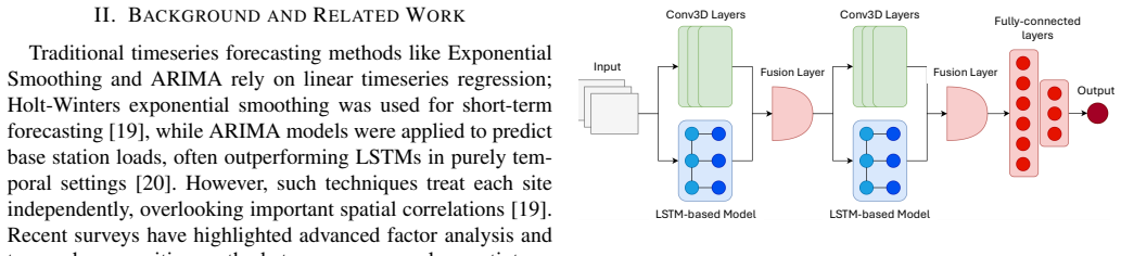
The central machinery is the scalar LSTM (sLSTM), a recurrent cell from the xLSTM family whose input and forget gates are scalar and exponentially gated, backed by multiple memory cells; it replaces ConvLSTM as the temporal branch. A three-layer Conv3D module supplies the spatial branch, and a transformer fusion layer computes cross-attention with spatial outputs as queries and temporal outputs as keys and values, replacing the original STN's linear fusion. The sLSTM carries temporal dependencies, the Conv3D captures local spatiotemporal patches, and the fusion layer adaptively combines the two streams before an MLP decodes the forecast.
What would settle it
Open the evaluation pipeline and check whether Trentino normalization uses Milan-derived statistics or Trentino's own per-cell statistics; then rerun the Trentino test with Milan statistics applied to Trentino data and see whether STN-sLSTM's MAE advantage (1.68 versus 2.63) over STN persists. Additionally, compare gradient norms or convergence curves of sLSTM against ConvLSTM to test the gradient-stability claim directly.
Extended reading notes
Core claim
On the paper's own reporting, replacing ConvLSTM with sLSTM in the temporal branch and switching the fusion from a linear layer to transformer cross-attention yields the best overall spatiotemporal forecaster among the tested variants. STN-sLSTM-TF reaches a single-step MAE of 5.5375 on Milan versus 7.3917 for the original STN, a 23% reduction, and on the unseen Trentino generalization test both sLSTM variants beat all baselines, with STN-sLSTM-TF achieving an R2 score of 0.9580. The authors attribute the gains to sLSTM's exponential gating and scalar state updates, which they say stabilize gradients and improve convergence, and to cross-attention fusion that lets spatial features query temporal context, which they say helps track high-magnitude peaks and preserve spatial structure over longer horizons.
Load-bearing premise
The generalization claim rests on how per-cell normalization is applied to Trentino: if each Trentino cell is normalized with its own mean and standard deviation rather than with statistics from Milan, the reported MAE and RMSE improvements on unseen data largely measure shape-transfer, not scale-transfer.
Editorial extensions
If this is right
- If the central claim is correct, swapping ConvLSTM for sLSTM in a dual-path spatiotemporal network yields consistently lower one-step and multi-step forecast errors on the Italia Telecom dataset.
- The reported 30% generalization improvement implies that a model trained on one urban region (Milan) can be applied directly to a different region (Trentino) without retraining, with MAE around 1.68 to 2.13 versus 2.63 for the original STN.
- The sLSTM variants preserve SSIM above 0.94 across six autoregressive steps on unseen Trentino, meaning spatial structure is still captured at a 60-minute horizon.
- Transformer fusion adds modest accuracy gains and better RMSE and R2 in high-traffic areas, but at a cost of roughly 4x the multiply-accumulate operations and about 10x the grid-level inference latency of the original STN.
- Cell-level inference time stays below 10 ms across all variants, which the paper argues keeps the model within near-real-time control-loop requirements even if grid-level latency is high.
Reading between the lines
- The reported Trentino gains may partly reflect per-cell normalization: since the paper says data are normalized per cell but does not state whether Trentino normalization uses Milan statistics or Trentino's own, the MAE and RMSE on Trentino could measure shape transfer rather than absolute traffic-scale transfer; a fair transfer test would normalize Trentino with Milan-derived parameters.
- The comparison set is limited to the STN family, plain LSTM, and xLSTM; the 23% MAE reduction is relative to those baselines, and the paper itself lists graph-based, transformer, and diffusion-hybrid spatiotemporal models as future benchmarks.
- The gradient-stability claim is supported by training-loss numbers but not by direct gradient measurements; comparing gradient norms or convergence curves of sLSTM versus ConvLSTM would test it explicitly.
- The grid-level latency of STN-sLSTM-TF (326 ms) suggests that real-world deployment would need horizontal scaling or pruning, an operational consequence the paper notes but does not quantify.
Signed reviews
Editorial analysis
A structured set of objections, weighed in public.
Referee Report
Summary. The paper proposes STN-sLSTM-TF, a spatiotemporal traffic forecasting architecture that replaces the ConvLSTM temporal branch of the original STN with a scalar LSTM (sLSTM) and replaces linear fusion with transformer cross-attention. Experiments on the Italia Telecom dataset (Milan training, Trentino as an unseen test region) report that the proposed model achieves a 23% MAE reduction over a ConvLSTM-based baseline and a 30% improvement in generalization to the unseen region. The paper also presents ablation studies isolating the sLSTM branch and the transformer fusion, and an autoregressive multi-step evaluation.
Significance. If the claimed results hold, the paper would contribute a practical, lightweight alternative to ConvLSTM-based spatiotemporal forecasting, with a clear ablation demonstrating the contribution of each architectural component. The use of a large public dataset with a held-out geographic region for generalization testing is a valuable experimental design. However, the strength of the claims is currently limited by an unspecified normalization protocol for the unseen region, missing statistical uncertainty estimates, and an inconsistent baseline statement for the headline 23% figure. The central generalization claim is not verifiable as reported, and the accuracy claim lacks error bars.
major comments (5)
- [Section IV-C2, Table III] Section IV-B2 states 'Data are normalized per cell' but never specifies whether the unseen Trentino region is normalized using Trentino's own per-cell statistics or statistics computed from Milan. This is load-bearing for the generalization claim in Section IV-D and Table V. If each Trentino cell is standardized with its own mean and standard deviation, the model is effectively provided with the target cell's marginal statistics at test time; a trivial mean-predictor would then achieve low absolute MAE/RMSE after inverse transformation, and the reported '30% improvement in model generalization' would largely measure scale invariance rather than learned transfer. Please state the exact normalization provenance for the Trentino evaluation and, if Trentino statistics were used, re-evaluate the generalization claim with a protocol that does not leak target-region statistics (e.g., using Milan statistics to transform Trentino, or reporting errors in normalized units).
- [Section IV-C2, Table III] The abstract and conclusion claim a '23% MAE reduction over ConvLSTM' (conclusion says 'over the original STN'). In Table III, the MAE reduction from STN-TF (7.2104) to STN-sLSTM-TF (5.5375) is 23.2%, while the reduction from the original STN (7.3917) is 25.1%; ConvLSTM itself is not evaluated as a standalone baseline. The 23% figure therefore appears to refer to the comparison with STN-TF, not with the original STN or with ConvLSTM. Please identify the exact baseline used for the headline number and correct the abstract and conclusion accordingly.
- [Sections IV-C2 and IV-D, Tables III and V] All test metrics are reported as single-run point estimates without variance or significance testing. In Table III, the advantage of STN-sLSTM-TF over STN-sLSTM is small (MAE 5.5375 vs 5.6319, SSIM 0.9921 vs 0.9912), and in Table V STN-sLSTM achieves lower MAE (1.6803 vs 2.1257) but higher RMSE (5.3016 vs 5.2649) than STN-sLSTM-TF. Without multiple seeds, confidence intervals, or a paired significance test, the claimed superiority of the full model over its closest variant is not statistically established. Please report runs over several seeds and include error bars or significance tests for the main comparisons.
- [Section IV-B2] The data split description is internally inconsistent: 'Models train on 1 million samples (70% of Milan, stride = 6) and test on 7 million samples (15% of Milan, stride = 1)' cannot both be true for the same dataset. If the total is 8.928 (million) samples, 70% is about 6.25 million and 15% is about 1.34 million, not 1 million and 7 million. Please clarify the actual number of training and test samples, the fraction they represent, and the stride definitions so that the evaluation protocol is reproducible.
- [Table I] The Milan quartile statistics in Table I are internally inconsistent: the 50th percentile is listed as 64.178 while the 25th percentile is 413.368, which is impossible for an ordered distribution. This appears to be a typo (perhaps 641.78 for the median). Since the table motivates the per-cell normalization and the regional disparity argument, the statistics must be corrected and verified.
minor comments (5)
- [Section III-B1 and Eq. (5)] The neighborhood size notation is inconsistent: the text says 'local region of size (r + 1) × (r + 1)' but Eq. (5) writes entries from x^{(i-r/2, j-r/2)} to x^{(i+r/2, j+r/2)}. For r = 5, r/2 = 2.5, which is not an integer; please use a consistent indexing scheme (e.g., i-r to i+r with kernel size 2r+1) and specify the exact patch boundaries.
- [Table II] The column header 'Gap (Ovr)' is not defined in the caption or text; it appears to be the difference between validation loss and best loss (an overfitting indicator), but this should be stated explicitly.
- [Section IV-B2] The 'Number of samples 8.928' in Table I lacks units; if it represents millions of samples, please state that explicitly, as it is essential for interpreting the 1M/7M sample split described later.
- [Section III-B1] The description of sLSTM is brief and does not provide the exact gating equations or memory-cell configuration; please either include the relevant sLSTM equations or give a precise pointer to the corresponding section in the xLSTM paper [18], so that the model is fully specified.
- [Section V] The conclusion states 'Empirical results showed a 23% MAE reduction over the original STN' while the abstract says 'over ConvLSTM baselines'; these two statements are not consistent with each other or with Table III. Please unify the wording after clarifying the baseline.
Circularity Check
No circularity; the model performance claims rest on held-out benchmarks and external baseline components.
full rationale
This paper makes no formal derivation claim; it reports empirical comparisons of architectures on a held-out test set and an unseen region. The proposed STN-sLSTM-TF model is assembled from published building blocks (sLSTM from the xLSTM paper [18], Conv3D modules, and transformer cross-attention), and its accuracy is evaluated with standard MAE, RMSE, R2, and SSIM metrics against baselines. No fitted parameter is later renamed as a prediction, and no equation defines the output in terms of its own target. The ablation variants share hyperparameters obtained from tuning the full STN-sLSTM-TF model with Optuna, and the Trentino generalization experiment does not state whether normalization statistics come from Milan or Trentino; both are experimental-design caveats that affect attribution and generalization claims, but neither makes the reported reductions equal to an input by construction. The citations to STN and xLSTM are external prior work, not unverified self-citations, and the central accuracy claim is benchmarked rather than derived from those references. Therefore no circular step is identified.
Assumptions & free parameters
free parameters (8)
- local patch radius r = 5 (11x11 kernel) =
r = 5
- number of past timesteps n = 6 =
6
- training sample stride = 6 =
6
- hidden size h = 64 =
64
- number of STN blocks b = 2 =
2
- sLSTM heads a = 4 =
4
- sLSTM layers l = 2 =
2
- fusion transformer heads f = 8 =
8
assumptions (4)
- domain assumption Local spatial factorization: p(X_{t+1} | past) approximately factorizes over cells and each cell depends only on its (r+1) x (r+1) neighborhood (Eq. 4).
- domain assumption Grid-level stationarity after spatial aggregation, confirmed by an Augmented Dickey-Fuller test, makes a fixed-window supervised learning setup valid.
- domain assumption sLSTM can be substituted for ConvLSTM in the temporal branch without changing the spatial branch interface, and its gradient-stability properties carry over.
- ad hoc to paper Per-cell normalization produces comparable error units across Milan and Trentino despite large differences in mean traffic (95.9 vs 622.0).
Cite this review
Pith. "Pith review of Enhancing Spatiotemporal Networks with xLSTM: A Scalar LSTM Approach for Cellular Traffic Forecasting." pith.science (2026). https://pith.science/paper/WQVKFTPB
@misc{pith2026250719513,
  author       = {Pith},
  title        = {Pith review of: Enhancing Spatiotemporal Networks with xLSTM: A Scalar LSTM Approach for Cellular Traffic Forecasting},
  year         = {2026},
  howpublished = {\url{https://pith.science/paper/WQVKFTPB}},
  note         = {Machine review of arXiv:2507.19513}
}
read the original abstract
Accurate spatiotemporal traffic forecasting is vital for intelligent resource management in 5G and beyond. However, conventional AI approaches often fail to capture the intricate spatial and temporal patterns that exist, due to e.g., the mobility of users. We introduce a lightweight, dual-path Spatiotemporal Network that leverages a Scalar LSTM (sLSTM) for efficient temporal modeling and a three-layer Conv3D module for spatial feature extraction. A fusion layer integrates both streams into a cohesive representation, enabling robust forecasting. Our design improves gradient stability and convergence speed while reducing prediction error. Evaluations on real-world datasets show superior forecast performance over ConvLSTM baselines and strong generalization to unseen regions, making it well-suited for large-scale, next-generation network deployments. Experimental evaluation shows a 23% MAE reduction over ConvLSTM, with a 30% improvement in model generalization.
Figures


Figures from the paper (4 more)




Reference graph
Works this paper leans on
-
[1]
Intelligent traffic adaptive resource allocation for edge computing-based 5g networks,
M. Chen, Y . Miao, H. Gharavi, L. Hu, and I. Humar, “Intelligent traffic adaptive resource allocation for edge computing-based 5g networks,” IEEE Transactions on Cognitive Communications and Networking, vol. 6, no. 2, pp. 499–508, 2020. [Online]. Available: https://doi.org/10.1109/TCCN.2019.2953061
arXiv 2020
-
[2]
Predictive uav base station deployment and service offloading with distributed edge learning,
Z. Zhao, L. Pacheco, H. Santos, M. Liu, A. D. Maio, D. Ros ´ario, E. Cerqueira, T. Braun, and X. Cao, “Predictive uav base station deployment and service offloading with distributed edge learning,” IEEE Transactions on Network and Service Management , vol. 18, no. 4, pp. 3955–3972, 2021. [Online]. Available: https://doi.org/10.1109/TNSM.2021.3123216
-
[3]
Millimeter-wave base station deployment using the scenario sampling approach,
M. Dong, T. Kim, J. Wu, and E. W.-M. Wong, “Millimeter-wave base station deployment using the scenario sampling approach,” IEEE Transactions on Vehicular Technology, vol. 69, no. 11, 2020. [Online]. Available: https://doi.org/110.1109/TVT.2020.3022744
-
[4]
W. Mei and R. Zhang, “Joint base station and irs deployment for enhancing network coverage: A graph-based modeling and optimization approach,” IEEE Transactions on Wireless Communications , vol. 22, no. 11, pp. 8200–8213, 2023. [Online]. Available: https://doi.org/110.1109/TWC.2023.3271234
-
[5]
G. E. Box, G. M. Jenkins, G. C. Reinsel, and G. M. Ljung, Time series analysis: forecasting and control . John Wiley & Sons, 1976
work page 1976
-
[6]
S. Hochreiter and J. Schmidhuber, “Long short-term memory,” Neural Computation, vol. 9, no. 8, pp. 1735–1780, 11 1997. [Online]. Available: https://doi.org/10.1162/neco.1997.9.8.1735
-
[7]
Lstm fully convolutional networks for time series classification,
F. Karim, S. Majumdar, H. Darabi, and S. Chen, “Lstm fully convolutional networks for time series classification,” IEEE Access, vol. 6, pp. 1662–1669, 2018. [Online]. Available: https://doi.org/10.1109/ACCESS.2017.2779939
-
[8]
Multivariate lstm-fcns for time series classification,
F. Karim, S. Majumdar, H. Darabi, and S. Harford, “Multivariate lstm-fcns for time series classification,” Neural Networks , vol. 116,
Show all 43 references
-
[9]
ROCKET: Exceptionally fast and accurate time series classification using random convolutional kernels,
A. Dempster, F. Petitjean, and G. I. Webb, “ROCKET: Exceptionally fast and accurate time series classification using random convolutional kernels,” Data Mining and Knowledge Discovery , vol. 34, no. 5, 2020. [Online]. Available: https://doi.org/10.1007/s10618-020-00701-z
2020 doi
-
[10]
Minirocket: A very fast (almost) deterministic transform for time series classification,
A. Dempster, D. F. Schmidt, and G. I. Webb, “Minirocket: A very fast (almost) deterministic transform for time series classification,” in Proceedings of the ACM SIGKDD Workshop on Mining and Learning from Time Series . ACM, 2021, pp. 248–257. [Online]. Available: https://doi.o...
2021
-
[11]
Temporal aggregation of univariate and multivariate time series models: A survey,
A. Silvestrini and D. Veredas, “Temporal aggregation of univariate and multivariate time series models: A survey,” Journal of Economic Surveys, vol. 22, no. 3, pp. 458–497, 2008. [Online]. Available: https://doi.org/10.1111/j.1467-6419.2007.00538.x
2008
-
[12]
The great multivariate time series classification bake off: A review and experimental evaluation of recent algorithmic advances,
A. P. Ruiz, M. Flynn, J. Large, M. Middlehurst, and A. Bagnall, “The great multivariate time series classification bake off: A review and experimental evaluation of recent algorithmic advances,” Data Mining and Knowledge Discovery , vol. 35, no. 2, pp. 401–449, 2021. [Online]....
2021 doi
-
[13]
Transformers in time series: a survey,
Q. Wen, T. Zhou, C. Zhang, W. Chen, Z. Ma, J. Yan, and L. Sun, “Transformers in time series: a survey,” in Proceedings of the 32nd International Joint Conference on Artificial Intelligence, 2023. [Online]. Available: https://doi.org/10.24963/ijcai.2023/759
2023 doi
-
[14]
Convolutional lstm network: a machine learning approach for precipitation nowcasting,
X. Shi, Z. Chen, H. Wang, D.-Y . Yeung, W.-k. Wong, and W.-c. Woo, “Convolutional lstm network: a machine learning approach for precipitation nowcasting,” in Proceedings of the 29th International Conference on Neural Information Processing Systems - Volume 1 , MA, USA, 2015, p...
2015
-
[15]
Long-term mobile traffic forecasting using deep spatio-temporal neural networks,
C. Zhang and P. Patras, “Long-term mobile traffic forecasting using deep spatio-temporal neural networks,” in Proceedings of the 18th ACM International Symposium on Mobile Ad Hoc Networking and Computing. NY , USA: Association for Computing Machinery, 2018, p. 231–240. [Online...
2018
-
[16]
Connecting the dots: Multivariate time series forecasting with graph neural networks,
Z. Wu, S. Pan, G. Long, J. Jiang, X. Chang, and C. Zhang, “Connecting the dots: Multivariate time series forecasting with graph neural networks,” in Proceedings of the 26th ACM SIGKDD International Conference on Knowledge Discovery & Data Mining . New York, NY , USA: Associati...
2020
-
[17]
Long-range transformers for dynamic spatiotemporal forecasting,
J. Grigsby, Z. Wang, and Y . Qi, “Long-range transformers for dynamic spatiotemporal forecasting,” 2021
2021
-
[18]
xlstm: Extended long short-term memory,
M. Beck, K. P ¨oppel, M. Spanring, A. Auer, O. Prudnikova, M. Kopp, G. Klambauer, J. Brandstetter, and S. Hochreiter, “xlstm: Extended long short-term memory,” in 38th Conference on Neural Information Processing Systems , 2024. [Online]. Available: https://arxiv.org/abs/2405.04517
2024 arXiv
-
[19]
Short-term traffic forecasting: Where we are and where we’re going,
E. I. Vlahogianni, M. G. Karlaftis, and J. C. Golias, “Short-term traffic forecasting: Where we are and where we’re going,” Transportation Research Part C: Emerging Technologies , vol. 43, pp. 3–19, 2014. [Online]. Available: https://doi.org/10.1016/j.trc.2014.01.005
2014 doi
-
[20]
Base station mobile traffic prediction based on arima and lstm model,
Y . Wang, “Base station mobile traffic prediction based on arima and lstm model,” in Proceedings of the 4th International Conference on Telecom- munications and Communication Engineering , M. Ma, Ed. Singapore: Springer Singapore, 2022, pp. 164–175
2022
-
[21]
A survey on deep learning for cellular traffic prediction,
X. Wang, Z. Wang, K. Yang, Z. Song, C. Bian, J. Feng, and C. Deng, “A survey on deep learning for cellular traffic prediction,” Intelligent Computing , vol. 3, p. 0054, 2024. [Online]. Available: https://doi.org/10.34133/icomputing.0054
2024 doi
-
[22]
Deep spatio-temporal adaptive 3d convolutional neural networks for traffic flow prediction,
H. Li, X. Li, L. Su, D. Jin, J. Huang, and D. Huang, “Deep spatio-temporal adaptive 3d convolutional neural networks for traffic flow prediction,” ACM Trans. Intell. Syst. Technol. , vol. 13, no. 2, Jan
-
[23]
Graph wavenet for deep spatial-temporal graph modeling,
Z. Wu, S. Pan, G. Long, J. Jiang, and C. Zhang, “Graph wavenet for deep spatial-temporal graph modeling,” in Proceedings of the 28th Inter- national Joint Conference on Artificial Intelligence, 2019, p. 1907–1913
2019
-
[24]
Stgformer: Efficient spatiotemporal graph transformer for traffic forecasting,
H. Wang, J. Chen, T. Pan, Z. Dong, L. Zhang, R. Jiang, and X. Song, “Stgformer: Efficient spatiotemporal graph transformer for traffic forecasting,” 2024. [Online]. Available: https://arxiv.org/abs/2410.00385
2024 arXiv
-
[25]
Citywide mobile traffic forecasting using spatial-temporal downsampling transformer neural networks,
Y . Hu, Y . Zhou, J. Song, L. Xu, and X. Zhou, “Citywide mobile traffic forecasting using spatial-temporal downsampling transformer neural networks,” IEEE Transactions on Network and Service Management , vol. 20, no. 1, p. 152–165, Mar. 2023. [Online]. Available: https://doi.o...
2023
-
[26]
Adaptive multi-receptive field spatial-temporal graph convolutional network for traffic forecasting,
X. Wang, J. Zhao, L. Zhu, X. Zhou, Z. Li, J. Feng, C. Deng, and Y . Zhang, “Adaptive multi-receptive field spatial-temporal graph convolutional network for traffic forecasting,” in IEEE Global Communications Conference . IEEE Press, 2021, p. 1–7. [Online]. Available: https://d...
2021
-
[27]
Joint spatial and temporal classi- fication of mobile traffic demands,
A. Furno, M. Fiore, and R. Stanica, “Joint spatial and temporal classi- fication of mobile traffic demands,” in IEEE INFOCOM 2017 - IEEE Conference on Computer Communications , 2017, pp. 1–9
2017
-
[28]
Understanding mobile traffic patterns of large scale cellular towers in urban environment,
H. Wang, F. Xu, Y . Li, P. Zhang, and D. Jin, “Understanding mobile traffic patterns of large scale cellular towers in urban environment,” in Proceedings of the Internet Measurement Conference . Association for Computing Machinery, 2015, pp. 225–238. [Online]. Available: https...
2015
-
[29]
The prediction analysis of cellular radio access network traffic: From entropy theory to networking practice,
R. Li, Z. Zhao, X. Zhou, J. Palicot, and H. Zhang, “The prediction analysis of cellular radio access network traffic: From entropy theory to networking practice,” IEEE Communications Magazine , vol. 52, no. 6, pp. 234–240, 2014
2014
-
[30]
Context- based interpretable spatio-temporal graph convolutional network for human motion forecasting,
E. Medina, L. Loh, N. Gurung, K. H. Oh, and N. Heller, “Context- based interpretable spatio-temporal graph convolutional network for human motion forecasting,” in 2024 IEEE/CVF Winter Conference on Applications of Computer Vision (WACV) , 2024, pp. 3220–3229
2024
-
[31]
Improving precipitation nowcasting using a three-dimensional convolutional neural network model from multi parameter phased array weather radar observations,
D.-K. Kim, T. Suezawa, T. Mega, H. Kikuchi, E. Yoshikawa, P. Baron, and T. Ushio, “Improving precipitation nowcasting using a three-dimensional convolutional neural network model from multi parameter phased array weather radar observations,” Atmospheric Research, vol. 262, p. ...
2021
-
[32]
Graph dual-stream convolutional attention fusion for precipitation nowcasting,
L. Vatam ´any and S. Mehrkanoon, “Graph dual-stream convolutional attention fusion for precipitation nowcasting,” Engineering Applications of Artificial Intelligence, vol. 141, p. 109788, 2025. [Online]. Available: https://doi.org/10.1016/j.engappai.2024.109788
2025
-
[33]
Residual networks behave like ensembles of relatively shallow networks,
A. Veit, M. Wilber, and S. Belongie, “Residual networks behave like ensembles of relatively shallow networks,” in Proceedings of the 30th International Conference on Neural Information Processing Systems . NY , USA: Curran Associates Inc., 2016, p. 550–558
2016
-
[34]
Attention is all you need,
A. Vaswani, N. Shazeer, N. Parmar, J. Uszkoreit, L. Jones, A. N. Gomez, L. Kaiser, and I. Polosukhin, “Attention is all you need,” in Proceedings of the 31st International Conference on Neural Information Processing Systems. NY , USA: Curran Associates Inc., 2017, p. 6000–6010
2017
-
[35]
Self-attention with relative position representations,
P. Shaw, J. Uszkoreit, and A. Vaswani, “Self-attention with relative position representations,” in Proceedings of the Conference of the North American Chapter of the Association for Computational Linguistics: Human Language Technologies, Volume 2 , M. Walker, H. Ji, and A. Ste...
2018 doi
-
[36]
Cross-modal attention for multi- modal image registration,
X. Song, H. Chao, X. Xu, H. Guo, S. Xu, B. Turkbey, B. J. Wood, T. Sanford, G. Wang, and P. Yan, “Cross-modal attention for multi- modal image registration,” Medical Image Analysis , vol. 82, p. 102612,
-
[37]
Layer normalization,
J. L. Ba, J. R. Kiros, and G. E. Hinton, “Layer normalization,” arXiv preprint arXiv:1607.06450 , 2016. [Online]. Available: https://arxiv.org/abs/1607.06450
2016 arXiv
-
[38]
Deep residual learning for image recognition,
K. He, X. Zhang, S. Ren, and J. Sun, “Deep residual learning for image recognition,” in Proceedings of the IEEE Conference on Computer Vision and Pattern Recognition (CVPR) , June 2016, p. 770–778. [Online]. Available: https://doi.org/10.1109/CVPR.2016.90
2016 doi
-
[39]
Available: https://doi.org/10.1016/j.media.2022.102612
[Online]. Available: https://doi.org/10.1016/j.media.2022.102612
2022
-
[40]
Adam: A method for stochastic optimization,
D. P. Kingma and J. Ba, “Adam: A method for stochastic optimization,” in 3rd International Conference on Learning Representations , Y . Bengio and Y . LeCun, Eds., 2015. [Online]. Available: https://arxiv.org/abs/1412.6980
2015 arXiv
-
[42]
A multi-source dataset of urban life in the city of milan and the province of trentino,
G. Barlacchi, M. De Nadai, R. Larcher, A. Casella, C. Chitic, G. Torrisi, F. Antonelli, A. Vespignani, A. Pentland, and B. Lepri, “A multi-source dataset of urban life in the city of milan and the province of trentino,” Scientific Data , vol. 2, no. 1, p. 150055, 2015. [Online...
2015 doi
-
[2019]
Available: https://doi.org/10.1016/j.neunet.2019.04.014
[Online]. Available: https://doi.org/10.1016/j.neunet.2019.04.014
2019 doi
- [2022]
Reviewed August 6, 2026 · model on record in the stance chip above.
Discussion (0). Continue with ORCID to comment.