Symplectic Neural Networks for learning Generalized Hamiltonians
Pith reviewed 2026-06-26 05:30 UTC · model grok-4.3
The pith
Symplectic discretizations of the adjoint system match backpropagation sensitivities to enable efficient training of implicit Hamiltonian Neural Networks.
A machine-rendered reading of the paper's core claim, the machinery that carries it, and where it could break.
Core claim
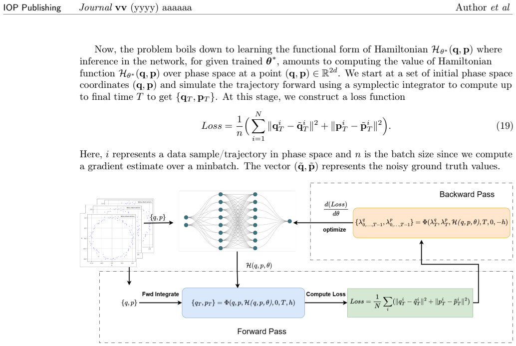
By leveraging the fact that symplectic discretizations of the adjoint system yield the same sensitivities associated by backpropagation, we obtain an efficient method of training the Neural Network parameters. In our work, we explore this alternate method of HNN training under noisy observation of trajectories with our HNN model based on an implicit symplectic integrator. Computationally, a predictor-corrector based ODE solver and fixed point iteration help to mitigate the computational cost of the implicit timestepping, resulting in more efficient generation of gradient updates. We showcase the numerical advantage, in experiments, in system identification and energy preservation on a range
What carries the argument
The equivalence between symplectic discretizations of the adjoint system and backpropagation sensitivities, which carries the argument by allowing gradient computation for implicit integrators without explicit differentiation through the solver.
If this is right
- Training of implicit symplectic HNNs becomes feasible with predictor-corrector solvers and fixed point iteration for gradient updates.
- Learned models achieve better system identification and energy preservation on non-separable chaotic systems than standard approaches.
- Backward error analysis post-processing produces a modified Hamiltonian that approximates the true one more closely without higher-order discretizations.
- Overall computation and memory complexity for gradient generation is reduced compared to direct backpropagation through implicit steps.
Where Pith is reading between the lines
- The sensitivity-matching property could extend to other structure-preserving integrators used in neural differential equations.
- Post-processed modified Hamiltonians might allow trading off discretization accuracy against correction steps in related geometric learning settings.
- The efficiency gains may support scaling the method to higher-dimensional physical systems where implicit methods were previously prohibitive.
Load-bearing premise
Fixed point iteration and predictor-corrector methods can efficiently solve the implicit equations without introducing significant errors that affect the learned Hamiltonian.
What would settle it
A numerical check on a simple known Hamiltonian where the symplectic adjoint gradients differ from standard backpropagation gradients, or where long-term energy drift in the learned model matches that of non-symplectic HNNs.
Figures





read the original abstract
Hamiltonian Neural Networks (HNNs) integrate physical priors into neural models by learning a system's Hamiltonian, improving generalization and sample efficiency. Identifying the system Hamiltonian from noisy observations of state variables is a challenging task. For simulations to faithfully reflect the long-term behavior of Hamiltonian systems, especially energy conservation, it is essential to use symplectic integrators, which preserve the system's geometric structure. This fidelity comes at a cost: implicit symplectic integrators are more computationally intensive and make backpropagation through the ODE solver non-trivial. However, by leveraging the fact that symplectic discretizations of the adjoint system yield the same sensitivities associated by backpropagation, we obtain an efficient method of training the Neural Network parameters. In our work, we explore this alternate method of HNN training under noisy observation of trajectories with our HNN model based on an implicit symplectic integrator. Computationally, a predictor-corrector based ODE solver and fixed point iteration help to mitigate the computational cost of the implicit timestepping, resulting in more efficient generation of gradient updates. We showcase the numerical advantage, in experiments, in system identification and energy preservation on a range of non-separable, chaotic systems and the efficient computation and memory complexity of our method. We also observe that the post-processing of the learned Hamiltonian using backward error analysis yields a modified Hamiltonian that is a more accurate approximation of the true Hamiltonian without the need to use more accurate discretizations of the flow map.
Editorial analysis
A structured set of objections, weighed in public.
Referee Report
Summary. The paper introduces Symplectic Neural Networks (SNNs) for learning generalized Hamiltonians from noisy trajectory observations. It replaces standard explicit integrators in HNNs with implicit symplectic ones, asserts that a symplectic discretization of the adjoint system produces identical parameter sensitivities to back-propagation through the flow map, and employs predictor-corrector schemes plus fixed-point iteration to keep the implicit steps tractable. Experiments on non-separable chaotic systems are reported to show improved long-term energy preservation and system identification; a post-processing step via backward error analysis is claimed to yield a modified Hamiltonian closer to the true one without requiring higher-order discretizations.
Significance. If the central equivalence between the symplectic discrete adjoint and back-propagation holds and the implicit solver residuals remain controlled, the method would make geometrically faithful integrators practical for HNN training, addressing a recognized computational bottleneck. The backward-error-analysis post-processing is a potentially useful, low-cost refinement. No machine-checked proofs or fully reproducible code artifacts are mentioned.
major comments (2)
- [Method / Implicit solver description] The central efficiency claim rests on the assertion that a finite number of fixed-point or predictor-corrector iterations produces a trajectory and discrete-adjoint gradient sufficiently close to the exact implicit symplectic step. No quantitative bound relating iteration count, residual norm, and gradient error is supplied, nor is an analysis given of how such residuals propagate under the chaotic dynamics highlighted in the experiments.
- [Adjoint discretization section] The statement that 'symplectic discretizations of the adjoint system yield the same sensitivities associated by backpropagation' is load-bearing for the entire training procedure. The manuscript must exhibit the precise discrete adjoint equations and demonstrate their equivalence to the chain-rule gradients through the implicit map; without this derivation the computational advantage cannot be verified.
minor comments (2)
- Notation for the learned Hamiltonian, the implicit map, and the modified Hamiltonian obtained by backward error analysis should be introduced once and used consistently.
- The experimental section would benefit from explicit reporting of iteration counts per time step and residual tolerances used in the fixed-point solver across all compared methods.
Simulated Author's Rebuttal
We thank the referee for the detailed and constructive report. We address each major comment below and commit to revisions that strengthen the manuscript without altering its core contributions.
read point-by-point responses
-
Referee: [Method / Implicit solver description] The central efficiency claim rests on the assertion that a finite number of fixed-point or predictor-corrector iterations produces a trajectory and discrete-adjoint gradient sufficiently close to the exact implicit symplectic step. No quantitative bound relating iteration count, residual norm, and gradient error is supplied, nor is an analysis given of how such residuals propagate under the chaotic dynamics highlighted in the experiments.
Authors: We agree that a quantitative analysis of residual propagation would improve rigor. In the revision we will add a dedicated subsection on the fixed-point iteration, deriving a contraction-mapping bound on the residual after a fixed number of iterations and relating it to the gradient error via the implicit function theorem. We will also augment the experiments with a sensitivity study that varies iteration count on the chaotic test systems and reports the resulting variation in learned Hamiltonian accuracy and long-term energy drift. revision: yes
-
Referee: [Adjoint discretization section] The statement that 'symplectic discretizations of the adjoint system yield the same sensitivities associated by backpropagation' is load-bearing for the entire training procedure. The manuscript must exhibit the precise discrete adjoint equations and demonstrate their equivalence to the chain-rule gradients through the implicit map; without this derivation the computational advantage cannot be verified.
Authors: We will expand the Adjoint discretization section to include the full set of discrete adjoint equations for the chosen implicit symplectic scheme together with a self-contained derivation that shows step-by-step equivalence to the chain-rule gradients obtained by differentiating through the implicit map. This addition will make the claimed computational advantage directly verifiable. revision: yes
Circularity Check
No circularity; derivation leverages established symplectic adjoint equivalence
full rationale
The paper's central claim rests on the known mathematical property that symplectic discretizations of the adjoint system produce the same sensitivities as backpropagation through the flow map. This is invoked as an external fact to enable efficient training, not derived or fitted within the paper itself. No self-definitional steps, fitted inputs renamed as predictions, or load-bearing self-citations appear in the abstract or described method. The predictor-corrector and fixed-point approximations are presented as computational mitigations rather than part of a closed derivation loop. The overall approach is self-contained against external benchmarks on symplectic integrators and adjoint methods.
Axiom & Free-Parameter Ledger
axioms (1)
- domain assumption The underlying dynamical system is Hamiltonian.
Reference graph
Works this paper leans on
-
[1]
Marsden J and Ratiu T 1999Introduction to Mechanics and Symmetry2nd ed (Texts in Applied Mathematicsvol 17) (New York: Springer-Verlag) ISBN 9780387986436
-
[2]
Kang F and Meng-Zhao Q 1991Computer Physics Communications65173–187
-
[3]
Hand L N and Finch J D 1998Analytical mechanics(Cambridge: Cambridge University Press)
-
[4]
Sanz-Serna J M and Calvo M P 2018Numerical Hamiltonian ProblemsApplied Mathematics and Nonlinear Science (Mineola, NY: Courier Dover Publications)
-
[5]
Channell P J and Scovel C 1990Nonlinearity3231
-
[6]
Ruth R D 1983IEEE Transactions on Nuclear Science302669–2671 ISSN 0018-9499 21 IOP PublishingJournalvv(yyyy) aaaaaa Authoret al
-
[7]
Hairer E, Lubich C and Wanner G 2006Geometric Numerical Integration: Structure-preserving algorithms for ordinary differential equations2nd ed (Springer Series in Computational Mathematicsvol 31) (Berlin: Springer-Verlag)
-
[8]
Feng K and Qin M 2010Symplectic Geometric Algorithms for Hamiltonian Systems(Berlin: Springer Berlin Heidelberg)
-
[9]
Maslovskaya S and Ober-Blöbaum S 2024IFAC-PapersOnLine5885–90
-
[10]
Valperga R, Webster K, Turaev D, Klein V and Lamb J 2022 Learning reversible symplectic dynamicsLearning for Dynamics and Control Conference(PMLR) pp 906–916
2022
-
[11]
Zhong G and Marsden J E 1988Physics Letters A133134–139
-
[12]
Bertalan T, Dietrich F, Mezić I and Kevrekidis I G 2019Chaos: An Interdisciplinary Journal of Nonlinear Science29
-
[13]
Arnol’d V I 2013Mathematical methods of classical mechanicsvol 60 (Springer Science & Business Media)
-
[14]
Abraham R and Marsden J E 1978Foundations of Mechanics2nd ed (Reading, MA: Addison-Wesley) (with the assistance of Tudor Ratiu and Richard Cushman)
-
[15]
Greydanus S, Dzamba M and Yosinski J 2019Advances in neural information processing systems32
- [16]
- [17]
- [18]
- [19]
-
[20]
Šípka M, Pavelka M, Esen O and Grmela M 2023Journal of Physics A: Mathematical and Theoretical56495201
-
[21]
Khoo Z Y, Wu D, Low J S C and Bressan S 2024Physical Review E110044205
-
[22]
Wu X, Wang Y, Sun W, Liu F and Ma D 2024The Astrophysical Journal Supplement Series 27531
- [23]
-
[24]
David M and Méhats F 2023Journal of Computational Physics494112495
-
[25]
Hairer E, Hochbruck M, Iserles A and Lubich C 2006Oberwolfach Reports3805–882
-
[26]
Yoshida H 1990Physics letters A150262–268
- [27]
-
[28]
Tao M 2016Physical Review E94043303
-
[29]
Rahma A, Datar C and Dietrich F 2024arXiv preprint arXiv:2411.17511URL https://arxiv.org/abs/2411.17511
work page internal anchor Pith review Pith/arXiv arXiv
-
[30]
Jin P, Zhang Z, Zhu A, Tang Y and Karniadakis G E 2020Neural Networks132166–179
-
[31]
Hairer E, Lubich C and Wanner G 2003Acta numerica12399–450
-
[32]
Leok M and Zhang J 2011IMA Journal of Numerical Analysis311497–1532
-
[33]
Barrio R and Wilczak D 2020Nonlinear Dynamics102403–416
-
[34]
Bolte J and Pauwels E 2021Mathematical Programming18819–51 22
discussion (0)
Sign in with ORCID, Apple, or X to comment. Anyone can read and Pith papers without signing in.