REVIEW 3 major objections 7 minor 16 references
Fixed-Confidence Multiple Change Point Identification under Bandit Feedback
T0 review · 3 major / 7 minor · reviewed 2026-08-06 · deepseek-v4-flash
Pith's one-line read This paper proves that locating $N$ jumps in a noisy piecewise-constant function can be done with $8\sigma^2\log(1/\delta)\sum_{i=1}^N 1/\Delta_i^2$ samples, and gives an algorithm that achieves it.
desk verdict Worth engaging: the lower bounds are solid, but the MCPI pseudocode has a control-flow bug that invalidates the stated theorem for N≥2, and the tie case breaks the non-asymptotic bound. read the letter →
The pith
A machine-rendered reading of the paper's core claim, the machinery that carries it, and where it could break.
The reading
What carries the argument
The load-bearing object is the explicit solution of the allocation game that defines the lower bound. Rather than solving a linear program every round, the paper shows the optimal proportions are supported only on the two arms flanking each change point, with weights proportional to inverse squared jump size; this turns Track-and-Stop into a simple rule. In each phase, MCPI estimates the current change point as the adjacent pair with the largest empirical mean difference, forces every arm to be played at least $\sqrt{t}$ times, tracks the less-played arm of the current pair, and stops when $Z(t) = T_{\hat{x}}T_{\hat{x}+1}\big/\big(2(T_{\hat{x}}+T_{\hat{x}+1})\big)\,\hat{\Delta}_{\hat{x}}^2$ crosses $\beta(t,\delta/N)$. The stopping statistic is itself a closed-form minimal KL divergence, so correctness can be checked directly without numerical optimization.
What would settle it
Simulate MCPI in the paper's two-change environment from Appendix A (changes of size 2 and 4) at $\delta = 10^{-8}, 10^{-10}, 10^{-12}$ and extrapolate $\mathbb{E}[\tau_\delta]/\log(1/\delta)$; Theorem 5.7 predicts convergence to $8(1/4+1/16)=5/2$, and a clear departure would refute the upper bound. To probe the unrelaxed separation assumption, run the same experiment on the adjacent-jump environment with means $(0,1,0)$; the stated lower bound and tracking analysis do not cover that case, so an observed ratio away from the predicted additive constant would show where the claim ends.
Extended reading notes
Core claim
On the paper's own terms, the discovery is that change-point identification under bandit feedback has a closed-form complexity and a matching algorithm. For a single change of size $\Delta$, the optimal proportion vector is $\alpha^*_i = 1/2$ at the two arms $x^*$ and $x^*+1$ and zero everywhere else, making the optimal constant $1/c^*(v) = \Delta^2/(8\sigma^2)$; for multiple changes with unknown total, the optimal allocation concentrates each change's samples on its two adjacent arms in proportion to $1/\Delta_i^2$. Theorem 5.7 states that MCPI is an Exact-$(N,\delta)$ and Any-$(N,\delta)$ policy with $\limsup_{\delta\to 0} \mathbb{E}_{\pi,v}[\tau_\delta]/\log(1/\delta) \le 8\sigma^2\sum_{i=1}^N 1/\Delta_{(i)}^2$, matching the lower bound of Theorem 5.5. Thus identifying any $N$ changes out of an unknown larger set is solved up to the asymptotic constant; the known-$N$ objective is matched up to a factor of two, and the known single-change case exactly.
Load-bearing premise
Everything rests on change points being separated by at least one action, $x^*_{v,i}+1 < x^*_{v,i+1}$; if two jumps are adjacent, the optimal-allocation decomposition and the tracking rule are not covered by the analysis.
Editorial extensions
If this is right
- A jump of half the size costs four times as many samples, since the complexity sums $1/\Delta_i^2$; small jumps dominate the budget.
- Sampling anywhere except the two arms adjacent to a jump is asymptotically wasted, so the optimal experiment concentrates all queries at $N$ local pairs.
- Not knowing the true number of change points costs at most a factor of two: the Any-$(N,\delta)$ objective matches the lower bound, while the Exact-$(N,\delta)$ objective is matched up to a factor of two.
- The complexity is independent of the number of arms $K$, unlike best-arm identification, because the piecewise-constant structure lets each query inform the whole interval.
- The stopping rule can be evaluated in closed form at every round, so the method remains practical for large action spaces where per-round numerical optimization would be prohibitive.
Reading between the lines
- Dropping the separation assumption $x^*_{v,i}+1 < x^*_{v,i+1}$ is the natural stress test: with adjacent jumps the local two-arm neighborhoods overlap, and neither the additive complexity decomposition nor the tracking rule obviously survives; a finite-time blow-up there would delimit the theorem's boundary.
- The same $1/\Delta_i^2$ allocation suggests a fixed-budget counterpart in which samples are split across jumps in proportion to inverse squared magnitudes before any confidence threshold is reached.
- An 'all changes above $\epsilon$' objective looks reachable by running MCPI with an adaptive target count, since the lower bound is dominated by the $N$ largest jumps and smaller jumps contribute little.
- The closed-form stopping statistic resembles offline CUSUM/GLR tests but with adaptively chosen queries, so the paper effectively supplies an active, sequential version of those tests.
Editorial analysis
A structured set of objections, weighed in public.
Referee Report
Summary. The paper introduces a fixed-confidence piecewise constant bandit problem, where the learner sequentially queries arms in a finite action space with Gaussian noise and must confidently identify the locations of N change points in the mean reward function. Two objectives are considered: Exact-(N,δ), where the number of change points is known exactly, and Any-(N,δ), where the learner must find any N change points among an unknown total m ≥ N. The authors prove instance-dependent lower bounds on the expected sample complexity, show that optimal sampling concentrates on the two arms immediately adjacent to each change point with proportions inversely proportional to the squared jump size, and propose MCPI (Algorithm 2), a sequential Track-and-Stop variant. They claim MCPI is asymptotically optimal for the Any-(N,δ) objective (matching the lower bound constant) and within a factor of two for the Exact-(N,δ) objective. The paper also contains non-asymptotic upper bounds and synthetic experiments comparing MCPI with a clustering-bandit baseline.
Significance. If the main claims are correct, the paper provides a clean formulation of fixed-confidence change-point identification under bandit feedback, with explicit constants in both lower and upper bounds. The closed-form solution of the allocation optimization problem (equations (4) and (17)) is a genuine simplification relative to generic Track-and-Stop methods, and the lower bounds are proved by standard change-of-measure arguments. The claim of asymptotic optimality for the Any-(N,δ) objective would be a valuable contribution. However, the central algorithmic result is currently undermined by a control-flow bug in Algorithm 2 and by an incomplete treatment of tied change magnitudes; these issues affect the validity of Theorem 5.7 as stated. The theoretical framework and lower-bound techniques are nonetheless solid enough that the problems appear fixable in a revision.
major comments (3)
- [§5.3, Eq. (20), Proposition 5.6] The phase loop in Algorithm 2 does not reset Z(t), the current estimate, or the phase time when moving from phase j to phase j+1. After phase j exits the while loop, we have Z(t) ≥ β(t, δ/N). At the start of phase j+1 the same t, Z(t), and threshold are in force, so the while condition Z(t) < β(t, δ/N) is already false, the loop body is never executed, and line 17 adds the same change point again. Thus for N≥2 the returned set can contain duplicates and have cardinality strictly less than N, violating Definitions 5.1 and 5.3 and the guarantees claimed in Theorem 5.7. The proof of Proposition 5.6 and Lemma I.3 silently assumes that after one change point is identified the tracking estimate switches to a remaining change point, but line 9 is inside the while body and is never reached if the loop condition is false. This is a control-flow bug: the pseudocode does not implement the algorithm analyzed in the proofs. It is fixable by re-initializing the statistic (and, if needed, the candidate) at the start of each phase, but the manuscript must be revised accordingly.
- [Appendix J, proof of Theorem 5.7] The definition of T'_1(v) is not well-founded in the presence of ties at the boundary. If m>N and the (N+1)-th largest change satisfies Δ_(ℓ)=Δ_(N) (i.e., there is no next change strictly smaller than Δ_(N)), then the condition r(T) < (Δ_(N)−Δ_(ℓ))/4 = 0 can never hold and T'_1(v) = ∞, making the non-asymptotic bound in Proposition 5.6 vacuous. The paragraph labeled 'Edge Case (Multiple Equally Sized Changes)' claims that condition (19) handles ties, but (19) does not enter the definition of T'_1(v), and Lemma I.2 still relies on this T'_1(v). Ties are explicitly part of the Any-(N,δ) setting, so the proof needs a separate argument for tied magnitudes, for example by redefining the relevant event to allow any N of the largest changes or by introducing a convention for Δ_(N+1) when ties occur.
- [Appendix J, proof of Theorem 5.7] The asymptotic derivation of T0(δ) in Appendix J is not rigorous as written. The chain from T0(δ) ≤ T2(ϵ2)+T3(ϵ3)+min{ T : T(1−ϵ2) ≥ 8β(T,δ/N)(Σ+ϵ3) } to the final limsup bound replaces β(T,δ/N) by log(1/δ) inside a minimum over T without justifying the interchange of the limit and the minimum, and the displayed expression '1/log(1/δ) min{ T : T(1−ϵ2) ≥ 8 log(1/δ)(Σ+ϵ3) }' still depends on δ on both sides. A correct proof should fix T = 8 log(1/δ)(Σ+ϵ3)/(1−ϵ2), use the fact that β(T,δ/N)/log(1/δ) → 1, and then take limits in the correct order. This is the proof of the paper's main upper bound, so it needs to be made precise.
minor comments (7)
- [Appendix C, Section 4.1] The label 'Theorem 4.3' appears in Appendix C and in the text after Corollary 4.3, but the result is stated as Corollary 4.3; the numbering is inconsistent.
- [Section 3] There is a typo: 'the leaner' should be 'the learner'.
- [Appendix I, Lemma I.3] The phrase 'we get the restul in the lemma' contains a typo ('result').
- [Appendix A, Figures 3 and 4] The figure captions use 'MPCI' instead of 'MCPI'.
- [Section 5.3, Algorithm 2] The pseudocode should state explicitly what happens when condition (19) fails; currently the reader must infer that the estimate remains unchanged.
- [Section 3] The assumption that change points are separated by at least one action is stated but not discussed further; since the optimal sampling and the MCPI tracking rule play the two arms immediately adjacent to each change point, this assumption is essential and should be highlighted as a scope limitation.
- [Appendix D, Proposition 4.4] The application of Theorem 2 of Magureanu et al. (2014) to arrive at inequality (30) is plausible but the constant γ is only referenced, not derived in the appendix; a brief derivation would improve self-containedness.
Circularity Check
No significant circularity: lower bounds are change-of-measure arguments, the algorithm is a constructive Track-and-Stop variant, and self-citations are background only.
full rationale
The derivation chain is self-contained against its stated model. The lower bounds (Theorems 4.2, 5.2, 5.4, 5.5) are proved by standard change-of-measure / transportation arguments against explicitly constructed alternative environments in Appendices B, F, G, and H; the optimal proportions (4) and (17) are solved from the lower-bound optimization problems, not assumed as inputs. The upper bounds (Theorems 4.5 and 5.7) are proved from concentration events and forced-exploration tracking arguments in Appendices E and I, with the stopping threshold beta(t, delta) chosen to make a union-bound probability at most delta; the asymptotic constant 8 sigma^2 sum 1/Delta^2 is obtained by solving T0(delta), not by fitting the lower-bound coefficient. Citations to the authors' earlier fixed-budget paper (Lazzaro & Pike-Burke, 2025) and to Garivier & Kaufmann (2016) are background or standard technique and are not load-bearing for the central claim. The reviewer-flagged phase-loop control-flow concern in Algorithm 2, if valid, is a correctness gap between pseudocode and proof, not an equivalence of the claimed result to its own inputs; it does not constitute circular reasoning. No fitted parameter is renamed as a prediction, and no uniqueness theorem is imported from the authors to forbid alternatives.
Assumptions & free parameters
free parameters (1)
- gamma in stopping threshold beta(t, delta) =
2 e^(396/log 3)
assumptions (5)
- domain assumption Rewards are i.i.d. Gaussian with known variance sigma^2 = 1
- domain assumption Change points are separated by at least one action (x*_{v,i} + 1 < x*_{v,i+1})
- domain assumption The mean reward is stationary and exactly piecewise constant over the action set
- standard math Concentration inequalities from Magureanu et al. (2014) and Degenne et al. (2019) hold as stated
- standard math Bauer's Maximum Principle
Cite this review
Pith. "Pith review of Fixed-Confidence Multiple Change Point Identification under Bandit Feedback." pith.science (2026). https://pith.science/paper/YMDZXYWN
@misc{pith2026250708994,
  author       = {Pith},
  title        = {Pith review of: Fixed-Confidence Multiple Change Point Identification under Bandit Feedback},
  year         = {2026},
  howpublished = {\url{https://pith.science/paper/YMDZXYWN}},
  note         = {Machine review of arXiv:2507.08994}
}
read the original abstract
Piecewise constant functions describe a variety of real-world phenomena in domains ranging from chemistry to manufacturing. In practice, it is often required to confidently identify the locations of the abrupt changes in these functions as quickly as possible. For this, we introduce a fixed-confidence piecewise constant bandit problem. Here, we sequentially query points in the domain and receive noisy evaluations of the function under bandit feedback. We provide instance-dependent lower bounds for the complexity of change point identification in this problem. These lower bounds illustrate that an optimal method should focus its sampling efforts adjacent to each of the change points, and the number of samples around each change point should be inversely proportional to the magnitude of the change. Building on this, we devise a simple and computationally efficient variant of Track-and-Stop and prove that it is asymptotically optimal in many regimes. We support our theoretical findings with experimental results in synthetic environments demonstrating the efficiency of our method.
Figures

Figures from the paper (2 more)


Reference graph
Works this paper leans on
-
[1]
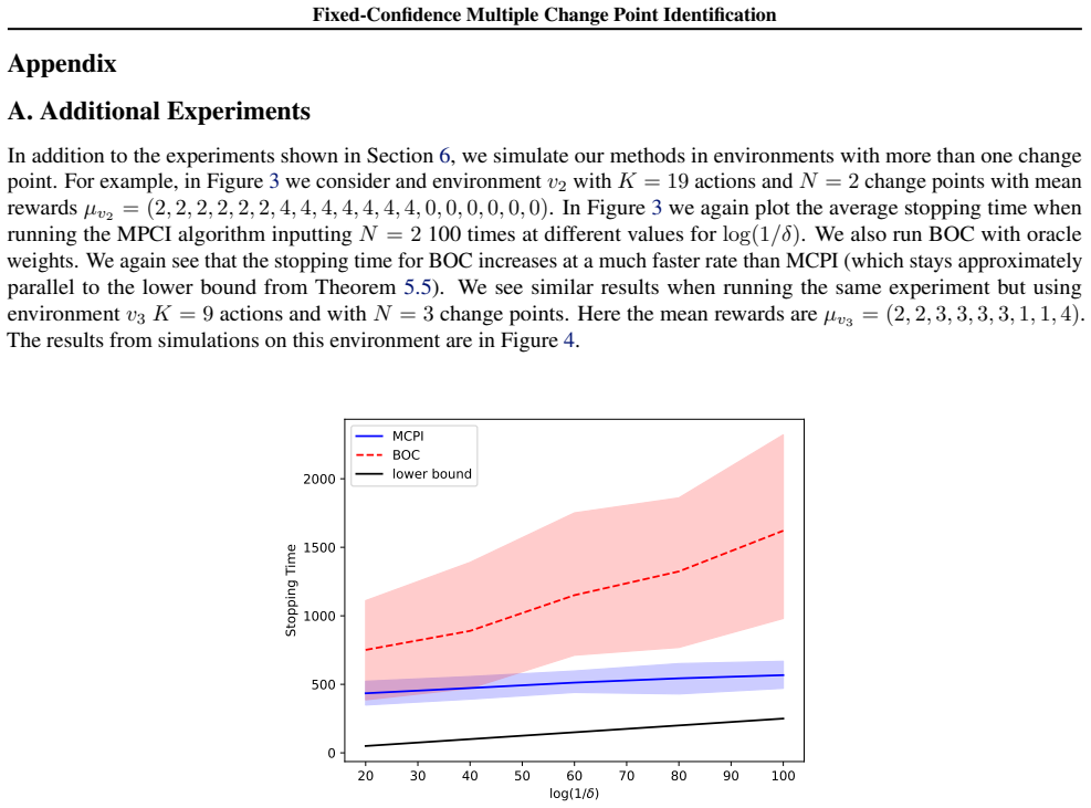
20 30 40 50 60 70 80 90 100 log(1/ ) 500 1000 1500 2000 2500Stopping Time MCPI lower bound Figure
We again see that the average stopping time of MCPI is approximately parallel to the lower bound, supporting our theoretical results that MCPI is an asymptotically optimal Any-(N, δ) policy which is robust to an unknown number of additional change points present in the environment. 20 30 40 50 60 70 80 90 100 log(1/ ) 500 1000 1500 2000 2500Stopping Time ...
work page 2000
-
[2]
and since β(t, δ/N) > β(s, δ/N); when ˜Zj(s) ≥ β(t, δ/N) occurs, we will never play actions x∗ (j) or x∗ (j) + 1 when tracking again. Hence, from (57), if Nj 4 (∆(j) − 2r(t))2 (58) holds then we will never play actions x∗ (j) or x∗ (j) + 1 when tracking again. By isolating the Nj values in (58) and summing through j ∈ [N ] (i.e. summing over the total num...
work page 2016
-
[3]
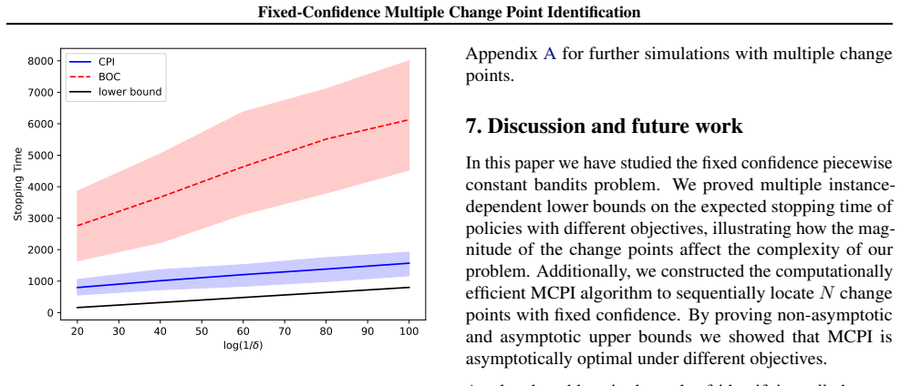
We run the MCPI and BOC algorithm at a range of values for δ in environment v2. At each confidence level we repeat 100 runs and plot the average stopping time with 90 percent confidence intervals. We also plot the lower bound in Theorem 5.5. 20 30 40 50 60 70 80 90 100 log(1/ ) 0 1000 2000 3000 4000 5000 6000 7000 8000Stopping Time MCPI BOC lower bound Figure
work page 2000
-
[6]
Active clustering with bandit feedback
URL https://arxiv.org/abs/2406.11485. Verzelen, N., Fromont, M., Lerasle, M., and Reynaud- Bouret, P. Optimal change-point detection and local- ization. The Annals of Statistics,
-
[10]
Case 2: Now, consider some v′ such that x∗ v′ < x∗ v. Similar to case 1, we can minimise the sum in (23) by setting µ′ 1 = µ1 µ′ K = µ1 + (µK − µ1) Px∗ v i=x∗ v′ +1 αi Px∗v i=x∗ v′ +1 αi + PK i=x∗v+1 αi x∗ v′ = x∗ v − 1 to attain 15 Fixed-Confidence Multiple Change Point Identification KX i=1 αiD(vi, v′ i) = ∆2 Px∗ v i=x∗ v′ +1 αi PK i=x∗v+1 αi 2σ2 Px∗v i...
work page 2016
-
[12]
Now, we will make similar arguments to Garivier et al
2 2 exp(−β(s, δ)) (30) Where (29) comes form the definition of our stopping time (28) and the final inequality (30) comes from Theorem 2 of (Magureanu et al., 2014). Now, we will make similar arguments to Garivier et al. (2018) to complete the proof. We first point out some helpful observations. Lemma D.1. The following inequalities hold for all t ≥ 1 and δ ∈ (0,
work page 2018
-
[13]
Furthermore, the inequality in (33) is true since we have γ(K − 1)/δ ≥ 3 from our definition of γ
2 log(3) (34) = δ Where equations (31) and (32) come from using the facts from Lemma D.1. Furthermore, the inequality in (33) is true since we have γ(K − 1)/δ ≥ 3 from our definition of γ. Inequality (34) is true by using an upper bounding integral. ∞X s=1 1 s log2(3s) ≤ 1 log2(3) + Z ∞ s=1 1 s log2(3s) = 1 log2(3) + 1 3log(3) ≤ 2 log(3) The final equatio...
work page 2016
-
[14]
exp (g(ϵ/8)) (37) Where for equation (37) we have used Lemma E.6. Hence, by plugging in the upper bound from (37) into (36), and observing the dependence of the upper bound on δ we attain the asymptotic upper bound stated in the theorem. Hence CPI has asymptotically optimal expected sample complexity. Helpful Lemma We state the following helpful lemma fro...
work page 2018
Show all 16 references
-
[15]
Where kl(x, y) is the KL-divergence between two Bernoulli distributions with parametersx and y
we have that D(P1, P2) ≥ kl(P1(A), P2(A)) ≥ 0 (44) for some event A. Where kl(x, y) is the KL-divergence between two Bernoulli distributions with parametersx and y. Recall also that kl(x, y) ≥ x log(1/y) − log(2) (45) Let v ∈ VK,m where m > Nand let π be an Any-(N, δ) policy. ...
1958
-
[1974]
Gaus- sian process optimization in the bandit setting: No re- gret and experimental design
Srinivas, N., Krause, A., Kakade, S., and Seeger, M. Gaus- sian process optimization in the bandit setting: No re- gret and experimental design. In ICML 2010 - Proceed- ings, 27th International Conference on Machine Learn- ing,
2010
-
[2014]
Sequential adaptive design for jump re- gression estimation
Park, C., Qiu, P., Carpena-N´u˜nez, J., Rao, R., Susner, M., and Maruyama, B. Sequential adaptive design for jump re- gression estimation. In ArXiv Preprint ArXiv:1904.01648,
1904 arXiv
-
[2016]
and Theorem 33.5 of (Lattimore & Szepesv´ari, 2020), where the difference is that we include additional structural assumptions on the mean rewards in our environments and we have a different objective from best arm identification. In particular, we reiterate the infimum in The...
2020
-
[2018]
URL https://arxiv.org/abs/1711. 04454. Gopalan, A., Lakshminarayanan, B., and Saligrama, V . Ban- dit quickest changepoint detection. Advances in Neu- ral Information Processing Systems 34 (NeurIPS 2021),
2021
-
[2020]
The general form of these stopping times are min ( t : inf v′∈V alt K,1(ˆx) KX i=1 Ti(t)D (v′(i), ˆv(i)) ≥ β(t, δ) )
crosses some threshold β. The general form of these stopping times are min ( t : inf v′∈V alt K,1(ˆx) KX i=1 Ti(t)D (v′(i), ˆv(i)) ≥ β(t, δ) ) . (27) where ˆv is an estimate for the environment. However, in our setting since it is optimal to only play either side of the change...
2020
-
[2021]
Active learning of piecewise gaussian process surrogates
Park, C., Waelder, R., Kang, B., Maruyama, B., Hong, S., and Gramacy, R. Active learning of piecewise gaussian process surrogates. In ArXiv Preprint ArXiv:2301.08789,
-
[2024]
and Nowak, R
Jamieson, K. and Nowak, R. Best-arm identification algo- rithms for multi-armed bandits in the fixed confidence setting. In 2014 48th Annual Conference on Information Sciences and Systems (CISS),
2014
Reviewed August 6, 2026 · model on record in the stance chip above.
Discussion (0). Continue with ORCID to comment.