REVIEW 4 major objections 4 minor 101 references
Investigating field burial by magnetically confined accretion mounds on Neutron Stars
T0 review · 4 major / 4 minor · reviewed 2026-08-06 · deepseek-v4-flash
Pith's one-line read Mound spreading buries neutron star dipole fields by up to 37 percent
desk verdict Useful methods paper with a genuinely new current-free BC; the 37% burial headline is real but resolution-bound, so treat it as evidence of onset, not a converged number. read the letter →
The pith
A machine-rendered reading of the paper's core claim, the machinery that carries it, and where it could break.
The reading
What carries the argument
The machinery is the axisymmetric, zero-toroidal-field Grad-Shafranov equation $\Delta_2 \psi = K(\psi,r,\theta)$ with $K = -4\pi r^2 \sin^2\theta\, \rho g\, dr_0/d\psi$, where $\psi$ is the poloidal flux function and $r_0(\psi)$ is a prescribed profile giving the height of each flux surface; for the ring-shaped mound, $r_0(\psi)$ is the inverted parabola of Eq. 16, which loads mass only up to the truncation angle $\theta_t$. The new ingredient is a multipolar current-free boundary condition (Eq. 15) that updates the outer radial boundary at every SOR iteration by decomposing the interior solution into associated Legendre multipoles ($\ell \le 33$) and matching to a source-free vacuum exterior, so the dipole and higher moments are free to evolve rather than being pinned to their surface values. This boundary condition is validated by showing that solutions become independent of the outer radius choice. The stretched radial coordinate ($y = \log((r-aR_*)/(R_*(1-a)))$ with $a=0.999$) and grid resolutions up to $5000^2$–$12000^2$ are what let the solver follow the large gradients at the mound edge and the subsequent equatorward spread.
What would settle it
Run the same GS solver while conserving $dM/d\psi$ between solutions, or perform a time-dependent axisymmetric MHD simulation of accretion onto a $10^9$ G neutron star with mass loaded up to $r_t = 0.6 R_A$, tracking the mound for hours: if the mound does not spread to the equator and the normalized dipole moment does not decline to about $0.627$, the burial result is an artifact of the assumed profile function.
Extended reading notes
Core claim
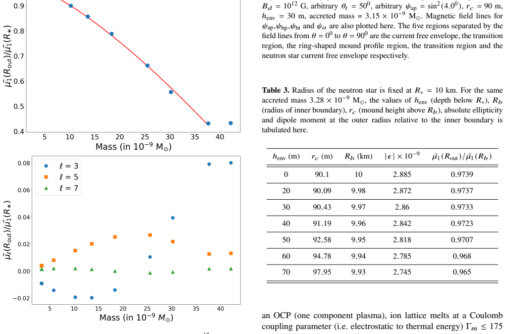
The paper's central claim is that magnetically confined accretion mounds, when computed at sufficient resolution with a boundary condition that lets multipoles evolve freely, do not hit a hard mass ceiling: instead the mound spreads equatorward as its mass grows, and this spreading is the physical mechanism of field burial. For a $10^9$ G neutron star with a mound loaded out to $r_t = 0.6 R_A$, the solution spreads all the way to the equator and the normalized dipole moment at the outer radius falls to $0.627$, a 37 percent reduction, with an octupole contribution rising to $0.12$. The paper argues this is the onset of field burial that earlier semi-analytic work anticipated, and that the closed magnetic loops which stopped previous solutions near $10^{-7}$–$10^{-8}$ M$\odot$ were numerical artifacts: they disappear at high resolution or with the ring-shaped profile, and the true limit is a resolution-dependent Numerical Maximum Mass beyond which solutions become non-unique. It also shows that the same physics applies when the mound sits on a pre-existing ocean, where sinking reduces ellipticity and dipole moment, and that quadru-dipolar surface fields make the two polar mounds asymmetric, with the asymmetry growing until matter funnels through the quadrupolar field.
Load-bearing premise
The equatorward spreading and the 37 percent dipole reduction depend on the hand-specified ring-shaped profile $r_0(\psi)$, which fixes the mass loading per flux surface; the paper explicitly does not impose a fixed $dM/d\psi$ between different solutions, so a physically self-consistent accretion model could yield a different profile and materially different burial efficiency.
Editorial extensions
If this is right
- For a $10^9$ G neutron star with $\zeta=0.6$, a mound accreted in about 9 hours spreads to the equator and cuts the normalized dipole moment to $0.627$, implying short-term field burial on outburst timescales.
- The resolution dependence of the Numerical Maximum Mass means published caps such as $10^{-7}$ M$\odot$ for a relativistic degenerate EOS are not physical limits; denser or better-resolved grids should push them higher.
- Mass ellipticity grows with accreted mass, reaching $\sim 3.75\times10^{-10}$ at $10^{12}$ G, and turns over once a mound spreads to the equator, a concrete signature for continuous gravitational wave searches.
- Mounds that sink into a pre-existing ocean retain most of their field-burial effect: with a helium composition and the crystallization-depth inner boundary, dipole reduction is slightly weaker and ellipticity is lower than for a pure hard-crust mound.
- Quadru-dipolar surface fields create asymmetric polar mounds with different heights and masses at the two poles, and beyond a field-dependent quadrupole fraction ($f_{qd} \gtrsim 1$ at $10^{10}$ G, $\gtrsim 5$ at $10^{12}$ G) accretion funnels directly through the quadrupolar field, outside the model's validity.
Reading between the lines
- The 37 percent burial figure is tied to the assumed $r_0(\psi)$; a self-consistent model that conserves $dM/d\psi$ between solutions could reduce or amplify the spreading, so the number should be read as a proof of mechanism rather than a precise prediction.
- If the current-free boundary result transfers to full time-dependent MHD, the same equator-ward spreading might operate in accreting millisecond pulsars on timescales of hours, making magnetic field evolution observable in a single outburst rather than over Gyr.
- The octupole enhancement (0.12 of the dipole) in the $10^9$ G burial case suggests that the surface field complexity inferred from X-ray pulse-profile modeling could be a direct signature of ongoing burial, not just an intrinsic multipole.
- The quadru-dipolar funneling limit predicts a qualitative change in accretion geometry, hot spots near the equator rather than the pole, which could be searched for in X-ray light curves of accreting pulsars with known field geometries.
Editorial analysis
A structured set of objections, weighed in public.
Referee Report
Summary. The paper solves the axisymmetric Grad-Shafranov (GS) equation for magnetically confined accretion mounds on neutron stars, using stretched spherical coordinates and a new multipolar current-free outer boundary condition. With a ring-shaped mound profile r0(psi) whose truncation angle is tied to the Alfven radius, the authors find that as mound mass increases, the mound spreads latitudinally toward the equator and the normalized dipole moment at the outer radius decreases. For B_d = 10^9 G and zeta = 0.6, the reported ratio is mu_1(Rout)/mu_1(R*) = 0.627, which they interpret as the onset of field burial. They also model mounds on a pre-existing ocean/envelope and quadrudipolar inner boundary configurations, which produce asymmetric polar mounds. The solver is validated against a Green's-function boundary condition (Appendix B3) and a perturbation-based uniqueness test defines a resolution-dependent Numerical Maximum Mass (NMM).
Significance. If the central result holds, the paper would overturn the common interpretation that closed magnetic loops set an intrinsic mass ceiling in GS mound calculations, and would support rapid field burial for low-field neutron stars in the early accretion phase. The new current-free boundary condition, the large parameter suite, the validation against a Green's-function volume boundary condition (relative difference below 5e-5 in Appendix B3), and the clearly described perturbation tests for numerical uniqueness are all valuable and reproducible contributions. However, because the headline dipole reduction is quoted at a resolution-limited numerical cutoff and the mass-loading profile is prescribed, the quantitative field-burial claim is not yet established as a converged physical prediction.
major comments (4)
- [Sec. 4.2.3, Table 5; Appendix C, Table C1] The central quantitative result, mu_1(Rout)/mu_1(R*) = 0.627 for B_d = 10^9 G and zeta = 0.6, is the value at the Numerical Maximum Mass, and NMM is not a physical mass limit. Table C1 shows that NMM increases monotonically with resolution, from 3.34e-13 M_sun at 700^2 to 5.65e-13 M_sun at 5000^2, and the text states that NMM is 'limited by resolution.' Because the dipole ratio decreases monotonically with accreted mass (Figs. 7 and 9), a higher-resolution run that supports a larger NMM could shift the ratio substantially below 0.627. The paper does not report how mu_1(Rout)/mu_1(R*) itself converges with resolution for this case, so the specific '37% reduction' is not a converged numerical prediction.
- [Sec. 2.5, Eq. (16); Limitations (ii)] The profile function r0(psi) in Eq. (16) is prescribed, and the limitations acknowledge that no fixed mass-loading per flux tube dM/dpsi is imposed between different solutions. Consequently, the sequence of solutions in Fig. 6 and the mass-dipole relations in Figs. 8-10 are not a single accretion sequence: each snapshot is an independent equilibrium with a different dM/dpsi. The equator-ward spreading and the 0.627 dipole ratio therefore measure properties of the chosen profile family, not of a physically self-consistent loading history. A model that fixes dM/dpsi during mound growth, or a detailed justification that the adopted r0(psi) follows from disk-magnetosphere interaction, is needed to support the field-burial interpretation.
- [Sec. 4.2.1; Limitations (v)] The text notes that matter beyond theta_t is supported by vacuum magnetic fields (or by a low-density envelope in the ocean model) and states that the dynamical stability of these spreading mounds should be verified. Since the central claim is that a mound can persist while spreading and burying the field, a static GS equilibrium alone does not demonstrate field burial unless the configuration is stable or the instability growth time exceeds the accretion time. Given the known interchange and pressure-driven instabilities of such mounds, the burial result should be presented conditional on a stability check.
- [Limitation (iv)] The authors report that general-relativistic GS solutions show approximately three times less screening than the Newtonian solutions (Rossetto et al. 2023). This directly affects the quantitative claim: the 37% reduction is a Newtonian value and may overestimate burial for the same mound parameters. The limitation is acknowledged, but the abstract and Section 4 present the Newtonian number without this caveat; the discussion in Section 6 should carry the GR caveat whenever the 0.627 figure is quoted.
minor comments (4)
- [Table 3] The column header 'R_b (km)' lists values such as 10, 9.98, and 9.93, which could be confused with R*; clarify that the dipole moment ratio in the last column is measured with respect to the inner boundary R_b, not the stellar surface.
- [Eq. (29)] The symbols alpha, epsilon, and h/r are used before their adopted values are introduced; the text should define these disk parameters explicitly when they first appear.
- [Eqs. (23), (25), (26)] These fits are empirical descriptions of the authors' own computed points; the text should state explicitly that they are not derived relations and should not be extrapolated outside the fitted mass and height ranges.
- [Sec. 4.1] The phrase 'Masses with an order of 10^-8 M_sun can be simulated' should read 'masses of order 10^-8 M_sun' to avoid grammatical ambiguity.
Circularity Check
No significant circularity: the dipole-moment ratios and ellipticities are computed outputs of the solved Grad–Shafranov equilibrium, not restatements of the prescribed profile functions.
full rationale
The derivation chain is: choose the EOS, the inner boundary field, the outer current-free boundary condition, the profile function r0(psi) (e.g. Eq. 16), and the mound height rc; solve Eq. 11 iteratively; then compute psi, from which Eq. 20 gives multipole moments and Eq. 22 gives ellipticity. The field-burial claims are readings of these converged numerical outputs (Figs. 6, 9, Table 5), not identities with the inputs. The hand-specified r0(psi) is an explicit modelling assumption, and the paper itself states the limitation that no fixed dM/dpsi between solutions is imposed, so the output mass distribution is not a hidden re-description of the input. The empirical fits in Eqs. 23, 25, and 26 are descriptive scalings of already-computed data and do not feed back into the central result. Self-citations to Mukherjee (2017) supply the ring-shaped profile and the Paczynski EOS as provenance for model choices; they are not invoked as an external uniqueness theorem that forces the outcome. The new current-free boundary condition is validated internally against a Green's-function volume boundary condition (Appendix B3) and by demonstrated domain-size independence (Figs. 3–4), so the boundary treatment is not circularly importing the dipole suppression. The resolution dependence of the Numerical Maximum Mass (Appendix C, Table C1) is an acknowledged numerical limitation that affects robustness of the quoted 37% reduction, but it is not a circularity: the NMM is defined by a perturbation-based uniqueness test applied to the solver, not by the quantity being predicted. No load-bearing step reduces by construction to its own inputs.
Assumptions & free parameters
free parameters (11)
- Ring profile shape constants (0.25, 0.5) =
0.25, 0.5
- Maximum mound height r_c =
Variable per run (e.g., 4.7 m to 103.1 m)
- Truncation angle theta_t =
Computed from Eq. 17 via Alfvén radius, or arbitrary (e.g., 50 deg)
- Truncation radius fraction zeta =
0.6, 0.7, 0.8, 0.9, 1.0
- Envelope depth h_env =
0 to 70 m
- Poleward boundary parameter psi_ap =
Corresponds to 4 deg
- Quadrupole to dipole fraction f_qd =
0.1, 1.0, 5.0
- Fit coefficients for dipole moment vs mass (Eq. 23) =
0.994, 0.00386, 1.376
- Fit coefficients for dipole moment and ellipticity vs h_env (Eqs. 25, 26) =
0.9739, 2.02e-8, 3.058 and 2.8835, 1.5e-5, 2.145
- Grid stretching parameter a =
0.999
- Quadrudipolar disk parameters alpha, h/r, epsilon =
0.1, 0.1, 1.0
assumptions (8)
- domain assumption Axisymmetry and zero toroidal magnetic field
- domain assumption Constant gravitational acceleration g = G M* / R*^2
- domain assumption Newtonian gravity
- domain assumption Paczynski EOS for zero-temperature degenerate electron gas
- domain assumption Fixed dipolar or quadrudipolar inner boundary
- ad hoc to paper Prescribed analytical profile function r0(psi)
- ad hoc to paper Current-free vacuum above R_in for the outer boundary condition
- domain assumption Quadrudipolar Alfvén radius prescription from Çıkıntoğlu (2023)
Cite this review
Pith. "Pith review of Investigating field burial by magnetically confined accretion mounds on Neutron Stars." pith.science (2026). https://pith.science/paper/ZIC2E7IG
@misc{pith2026250708509,
  author       = {Pith},
  title        = {Pith review of: Investigating field burial by magnetically confined accretion mounds on Neutron Stars},
  year         = {2026},
  howpublished = {\url{https://pith.science/paper/ZIC2E7IG}},
  note         = {Machine review of arXiv:2507.08509}
}
read the original abstract
We explore the problem of magnetic confinement of accreted matter forming an accretion mound near the magnetic poles of a neutron star. We calculate the magnetic field geometry of the accreted mound by solving the magnetostatic Grad Shafranov (GS) equation in radially stretched spherical coordinates with high resolution and an extended domain. In this work, we propose a new physically motivated multipolar current free boundary condition at the outer radial boundary. We have evaluated a large suite of GS solutions for different neutron star magnetic fields and mound configurations. We find that with sufficient resolution, the ring-shaped mound profiles spread latitudinally on the neutron star surface, towards the equator, with a potential decline in dipole moment at outer radii, demonstrating the onset of field burial. A higher latitudinal spread towards the equator leads to more effective magnetic field burial. Along with the ring-shaped mound profile on a hard crust majorly used in this work, we also model mounds formed on a pre-existing ocean, which is more physically motivated. Additionally, we explore different GS solutions for a quadru-dipolar surface magnetic field. We find that such configurations lead to asymmetric polar mounds. We discuss the validity of such solutions for different relative strengths of the quadrupole and dipolar components.
Figures


Figures from the paper (12 more)




Reference graph
Works this paper leans on
-
[1]
write newline
" write newline "" before.all 'output.state := FUNCTION fin.entry write newline FUNCTION new.block output.state before.all = 'skip after.block 'output.state := if FUNCTION new.sentence output.state after.block = 'skip output.state before.all = 'skip after.sentence 'output.state := if if FUNCTION not #0 #1 if FUNCTION and 'skip pop #0 if FUNCTION or pop #1...
-
[2]
Alford M. G., Schwenzer K., 2014, @doi [ ] 10.1088/0004-637X/781/1/26 , https://ui.adsabs.harvard.edu/abs/2014ApJ...781...26A 781, 26
-
[3]
Alpar M. A., Cheng A. F., Ruderman M. A., Shaham J., 1982, @doi [ ] 10.1038/300728a0 , https://ui.adsabs.harvard.edu/abs/1982Natur.300..728A 300, 728
doi:10.1038/300728a0 1982
-
[4]
M., 1976a, @doi [ ] 10.1086/154562 , https://ui.adsabs.harvard.edu/abs/1976ApJ...207..914A 207, 914
Arons J., Lea S. M., 1976a, @doi [ ] 10.1086/154562 , https://ui.adsabs.harvard.edu/abs/1976ApJ...207..914A 207, 914
-
[5]
M., 1976b, @doi [ ] 10.1086/154888 , https://ui.adsabs.harvard.edu/abs/1976ApJ...210..792A 210, 792
Arons J., Lea S. M., 1976b, @doi [ ] 10.1086/154888 , https://ui.adsabs.harvard.edu/abs/1976ApJ...210..792A 210, 792
-
[6]
M., 1980, @doi [ ] 10.1086/157706 , https://ui.adsabs.harvard.edu/abs/1980ApJ...235.1016A 235, 1016
Arons J., Lea S. M., 1980, @doi [ ] 10.1086/157706 , https://ui.adsabs.harvard.edu/abs/1980ApJ...235.1016A 235, 1016
-
[7]
Arumugasamy P., Mitra D., 2019, @doi [ ] 10.1093/mnras/stz2299 , https://ui.adsabs.harvard.edu/abs/2019MNRAS.489.4589A 489, 4589
-
[8]
Baym G., Pethick C., Pines D., Ruderman M., 1969, @doi [ ] 10.1038/224872a0 , https://ui.adsabs.harvard.edu/abs/1969Natur.224..872B 224, 872
doi:10.1038/224872a0 1969
Show all 101 references
-
[9]
A., Wolff M
Becker P. A., Wolff M. T., 2007, @doi [ ] 10.1086/509108 , https://ui.adsabs.harvard.edu/abs/2007ApJ...654..435B 654, 435
2007 doi
-
[10]
Bessolaz N., Zanni C., Ferreira J., Keppens R., Bouvier J., 2008, @doi [ ] 10.1051/0004-6361:20078328 , https://ui.adsabs.harvard.edu/abs/2008A&A...478..155B 478, 155
2008 doi
-
[11]
Bildsten L., 1998, @doi [ ] 10.1086/311440 , https://ui.adsabs.harvard.edu/abs/1998ApJ...501L..89B 501, L89
1998 doi
-
[12]
V., et al., 2019, @doi [ ] 10.3847/2041-8213/ab53e7 , https://ui.adsabs.harvard.edu/abs/2019ApJ...887L..23B 887, L23
Bilous A. V., et al., 2019, @doi [ ] 10.3847/2041-8213/ab53e7 , https://ui.adsabs.harvard.edu/abs/2019ApJ...887L..23B 887, L23
2019 doi
-
[13]
S., Komberg B
Bisnovatyi-Kogan G. S., Komberg B. V., 1974, , https://ui.adsabs.harvard.edu/abs/1974SvA....18..217B 18, 217
1974
-
[14]
D., Decampli W
Blandford R. D., Decampli W. M., Konigl A., 1979, in Bulletin of the American Astronomical Society. p. 703
1979
-
[15]
M., Freese K., 1986, @doi [ ] 10.1038/323786a0 , https://ui.adsabs.harvard.edu/abs/1986Natur.323..786B 323, 786
Blondin J. M., Freese K., 1986, @doi [ ] 10.1038/323786a0 , https://ui.adsabs.harvard.edu/abs/1986Natur.323..786B 323, 786
1986 doi
- [16]
-
[17]
F., Bildsten L., 1998, @doi [ ] 10.1086/305419 , https://ui.adsabs.harvard.edu/abs/1998ApJ...496..915B 496, 915
Brown E. F., Bildsten L., 1998, @doi [ ] 10.1086/305419 , https://ui.adsabs.harvard.edu/abs/1998ApJ...496..915B 496, 915
1998 doi
-
[18]
Caiazzo I., Heyl J., 2021, @doi [ ] 10.1093/mnras/staa3428 , https://ui.adsabs.harvard.edu/abs/2021MNRAS.501..109C 501, 109
2021 doi
-
[19]
Chandrasekhar S., 1970, @doi [ ] 10.1103/PhysRevLett.24.611 , https://ui.adsabs.harvard.edu/abs/1970PhRvL..24..611C 24, 611
1970 doi
-
[20]
Chatterjee D., Novak J., Oertel M., 2021, @doi [European Physical Journal A] 10.1140/epja/s10050-021-00525-5 , https://ui.adsabs.harvard.edu/abs/2021EPJA...57..249C 57, 249
2021 doi
-
[21]
Y., Yuan Y., Vasilopoulos G., 2020, @doi [ ] 10.3847/2041-8213/ab85c5 , https://ui.adsabs.harvard.edu/abs/2020ApJ...893L..38C 893, L38
Chen A. Y., Yuan Y., Vasilopoulos G., 2020, @doi [ ] 10.3847/2041-8213/ab85c5 , https://ui.adsabs.harvard.edu/abs/2020ApJ...893L..38C 893, L38
2020 doi
-
[22]
R., Konar S., 2002, @doi [ ] 10.1046/j.1365-8711.2002.05362.x , https://ui.adsabs.harvard.edu/abs/2002MNRAS.332..933C 332, 933
Choudhuri A. R., Konar S., 2002, @doi [ ] 10.1046/j.1365-8711.2002.05362.x , https://ui.adsabs.harvard.edu/abs/2002MNRAS.332..933C 332, 933
2002
-
[23]
A., Rothschild R
Coburn W., Heindl W. A., Rothschild R. E., Gruber D. E., Kreykenbohm I., Wilms J., Kretschmar P., Staubert R., 2002, @doi [ ] 10.1086/343033 , https://ui.adsabs.harvard.edu/abs/2002ApJ...580..394C 580, 394
2002 doi
-
[24]
Cumming A., Zweibel E., Bildsten L., 2001, @doi [ ] 10.1086/321658 , https://ui.adsabs.harvard.edu/abs/2001ApJ...557..958C 557, 958
2001 doi
-
[25]
Cutler C., 2002, @doi [ ] 10.1103/PhysRevD.66.084025 , https://ui.adsabs.harvard.edu/abs/2002PhRvD..66h4025C 66, 084025
2002 doi
-
[26]
L., 2022, @doi [ ] 10.1093/mnras/stac1817 , https://ui.adsabs.harvard.edu/abs/2022MNRAS.515.3144D 515, 3144
Das P., Porth O., Watts A. L., 2022, @doi [ ] 10.1093/mnras/stac1817 , https://ui.adsabs.harvard.edu/abs/2022MNRAS.515.3144D 515, 3144
2022 doi
- [27]
-
[28]
L., Schutz B
Friedman J. L., Schutz B. F., 1978, @doi [ ] 10.1086/156143 , https://ui.adsabs.harvard.edu/abs/1978ApJ...222..281F 222, 281
1978 doi
-
[29]
Fujisawa K., Kisaka S., Kojima Y., 2022, @doi [ ] 10.1093/mnras/stac2585 , https://ui.adsabs.harvard.edu/abs/2022MNRAS.516.5196F 516, 5196
2022 doi
-
[30]
Geppert U., 2017, @doi [Journal of Astrophysics and Astronomy] 10.1007/s12036-017-9460-y , https://ui.adsabs.harvard.edu/abs/2017JApA...38...46G 38, 46
2017 doi
-
[31]
Giliberti E., Cambiotti G., 2022, @doi [ ] 10.1093/mnras/stac245 , https://ui.adsabs.harvard.edu/abs/2022MNRAS.511.3365G 511, 3365
2022 doi
-
[32]
Goedbloed J. P. H., Poedts S., 2004, Principles of Magnetohydrodynamics
2004
-
[33]
Y., Yakovlev D
Haensel P., Potekhin A. Y., Yakovlev D. G., 2007, Neutron Stars 1 : Equation of State and Structure . Vol. 326, Springer New York, NY
2007
-
[34]
M., Bonazzola S., Heyvaerts J., Lasota J
Hameury J. M., Bonazzola S., Heyvaerts J., Lasota J. P., 1983, , https://ui.adsabs.harvard.edu/abs/1983A&A...128..369H 128, 369
1983
-
[35]
Haskell B., Antonelli M., Pizzochero P., 2022, @doi [Universe] 10.3390/universe8120619 , https://ui.adsabs.harvard.edu/abs/2022Univ....8..619H 8, 619
2022 doi
-
[36]
N., Semerikov I
Istomin Y. N., Semerikov I. A., 2016, @doi [ ] 10.1093/mnras/stv2473 , https://ui.adsabs.harvard.edu/abs/2016MNRAS.455.1938I 455, 1938
2016 doi
-
[37]
Jahan Miri M., Bhattacharya D., 1994, @doi [ ] 10.1093/mnras/269.2.455 , https://ui.adsabs.harvard.edu/abs/1994MNRAS.269..455J 269, 455
1994 doi
-
[39]
K., Kazanas D., 2021, @doi [ ] 10.3847/1538-4357/abcec0 , https://ui.adsabs.harvard.edu/abs/2021ApJ...907...63K 907, 63
Kalapotharakos C., Wadiasingh Z., Harding A. K., Kazanas D., 2021, @doi [ ] 10.3847/1538-4357/abcec0 , https://ui.adsabs.harvard.edu/abs/2021ApJ...907...63K 907, 63
2021 doi
-
[40]
D., Melatos A., 2022, @doi [ ] 10.1093/mnras/stac1351 , https://ui.adsabs.harvard.edu/abs/2022MNRAS.514.1628K 514, 1628
Kerin A. D., Melatos A., 2022, @doi [ ] 10.1093/mnras/stac1351 , https://ui.adsabs.harvard.edu/abs/2022MNRAS.514.1628K 514, 1628
2022 doi
-
[41]
Konar S., 2017, @doi [Journal of Astrophysics and Astronomy] 10.1007/s12036-017-9467-4 , https://ui.adsabs.harvard.edu/abs/2017JApA...38...47K 38, 47
2017 doi
-
[42]
Konar S., Bhattacharya D., 1997, @doi [ ] 10.1093/mnras/284.2.311 , https://ui.adsabs.harvard.edu/abs/1997MNRAS.284..311K 284, 311
1997 doi
-
[44]
Konar S., Bhattacharya D., 1999b, @doi [ ] 10.1046/j.1365-8711.1999.02781.x , https://ui.adsabs.harvard.edu/abs/1999MNRAS.308..795K 308, 795
1999
-
[46]
K., Romanova M
Kulkarni A. K., Romanova M. M., 2013, @doi [ ] 10.1093/mnras/stt945 , https://ui.adsabs.harvard.edu/abs/2013MNRAS.433.3048K 433, 3048
2013 doi
-
[47]
M., Sunyaev R., 2020, @doi [Journal of Plasma Physics] 10.1017/S0022377820001026 , https://ui.adsabs.harvard.edu/abs/2020JPlPh..86f9002K 86, 905860602
Kulsrud R. M., Sunyaev R., 2020, @doi [Journal of Plasma Physics] 10.1017/S0022377820001026 , https://ui.adsabs.harvard.edu/abs/2020JPlPh..86f9002K 86, 905860602
2020 doi
-
[48]
M., Prakash M., 2004, @doi [Science] 10.1126/science.1090720 , https://ui.adsabs.harvard.edu/abs/2004Sci...304..536L 304, 536
Lattimer J. M., Prakash M., 2004, @doi [Science] 10.1126/science.1090720 , https://ui.adsabs.harvard.edu/abs/2004Sci...304..536L 304, 536
2004 doi
-
[49]
Lindblom L., Mendell G., 1995, @doi [ ] 10.1086/175653 , https://ui.adsabs.harvard.edu/abs/1995ApJ...444..804L 444, 804
1995 doi
-
[50]
M., Lovelace R
Long M., Romanova M. M., Lovelace R. V. E., 2005, @doi [ ] 10.1086/497000 , https://ui.adsabs.harvard.edu/abs/2005ApJ...634.1214L 634, 1214
2005 doi
-
[51]
G., Melatos A., 2015, @doi [ ] 10.1093/mnras/stu2671 , https://ui.adsabs.harvard.edu/abs/2015MNRAS.447.3475M 447, 3475
Mastrano A., Suvorov A. G., Melatos A., 2015, @doi [ ] 10.1093/mnras/stu2671 , https://ui.adsabs.harvard.edu/abs/2015MNRAS.447.3475M 447, 3475
2015 doi
-
[52]
Melatos A., Payne D. J. B., 2005, @doi [ ] 10.1086/428600 , https://ui.adsabs.harvard.edu/abs/2005ApJ...623.1044M 623, 1044
2005 doi
-
[53]
S., 2001, @doi [ ] 10.1071/AS01056 , https://ui.adsabs.harvard.edu/abs/2001PASA...18..421M 18, 421
Melatos A., Phinney E. S., 2001, @doi [ ] 10.1071/AS01056 , https://ui.adsabs.harvard.edu/abs/2001PASA...18..421M 18, 421
2001 doi
-
[54]
A., Simula T
Melatos A., Douglass J. A., Simula T. P., 2015, @doi [ ] 10.1088/0004-637X/807/2/132 , https://ui.adsabs.harvard.edu/abs/2015ApJ...807..132M 807, 132
2015 doi
-
[55]
Mukherjee D., 2017, @doi [Journal of Astrophysics and Astronomy] 10.1007/s12036-017-9465-6 , https://ui.adsabs.harvard.edu/abs/2017JApA...38...48M 38, 48
2017 doi
-
[57]
Mukherjee D., Bhattacharya D., Mignone A., 2013a, @doi [ ] 10.1093/mnras/stt020 , https://ui.adsabs.harvard.edu/abs/2013MNRAS.430.1976M 430, 1976
1976 doi
-
[58]
Mukherjee D., Bhattacharya D., Mignone A., 2013b, @doi [ ] 10.1093/mnras/stt1344 , https://ui.adsabs.harvard.edu/abs/2013MNRAS.435..718M 435, 718
-
[59]
Mukherjee D., Bult P., van der Klis M., Bhattacharya D., 2015, @doi [ ] 10.1093/mnras/stv1542 , https://ui.adsabs.harvard.edu/abs/2015MNRAS.452.3994M 452, 3994
2015 doi
-
[60]
G., Tsygan A
Muslimov A. G., Tsygan A. I., 1985, Soviet Astronomy Letters, https://ui.adsabs.harvard.edu/abs/1985SvAL...11...80M 11, 80
1985
-
[61]
Mytidis A., Coughlin M., Whiting B., 2015, @doi [ ] 10.1088/0004-637X/810/1/27 , https://ui.adsabs.harvard.edu/abs/2015ApJ...810...27M 810, 27
2015 doi
-
[62]
a ttil \
N \"a ttil \"a J., Cho J. Y. K., Skinner J. W., Most E. R., Ripperda B., 2024, @doi [ ] 10.3847/1538-4357/ad54c2 , https://ui.adsabs.harvard.edu/abs/2024ApJ...971...37N 971, 37
2024 doi
-
[63]
Nazari E., Roshan M., 2020, @doi [ ] 10.1093/mnras/staa2322 , https://ui.adsabs.harvard.edu/abs/2020MNRAS.498..110N 498, 110
2020 doi
-
[64]
A., 1961, @doi [Physics of Fluids] 10.1063/1.1706342 , https://ui.adsabs.harvard.edu/abs/1961PhFl....4..391N 4, 391
Newcomb W. A., 1961, @doi [Physics of Fluids] 10.1063/1.1706342 , https://ui.adsabs.harvard.edu/abs/1961PhFl....4..391N 4, 391
1961 doi
-
[65]
J., 2010, @doi [ ] 10.1103/PhysRevD.82.104002 , https://ui.adsabs.harvard.edu/abs/2010PhRvD..82j4002O 82, 104002
Owen B. J., 2010, @doi [ ] 10.1103/PhysRevD.82.104002 , https://ui.adsabs.harvard.edu/abs/2010PhRvD..82j4002O 82, 104002
2010 doi
-
[66]
Paczynski B., 1983, @doi [ ] 10.1086/160870 , https://ui.adsabs.harvard.edu/abs/1983ApJ...267..315P 267, 315
1983 doi
-
[67]
R., Pines D., Smith R
Pandharipande V. R., Pines D., Smith R. A., 1976, @doi [ ] 10.1086/154637 , https://ui.adsabs.harvard.edu/abs/1976ApJ...208..550P 208, 550
1976 doi
-
[68]
Parfrey K., Tchekhovskoy A., 2017, @doi [ ] 10.3847/2041-8213/aa9c85 , https://ui.adsabs.harvard.edu/abs/2017ApJ...851L..34P 851, L34
2017 doi
-
[69]
M., 2017, @doi [ ] 10.1093/mnras/stx950 , https://ui.adsabs.harvard.edu/abs/2017MNRAS.469.3656P 469, 3656
Parfrey K., Spitkovsky A., Beloborodov A. M., 2017, @doi [ ] 10.1093/mnras/stx950 , https://ui.adsabs.harvard.edu/abs/2017MNRAS.469.3656P 469, 3656
2017 doi
-
[70]
Patruno A., 2012, @doi [ ] 10.1088/2041-8205/753/1/L12 , https://ui.adsabs.harvard.edu/abs/2012ApJ...753L..12P 753, L12
2012 doi
-
[71]
Payne D. J. B., Melatos A., 2004, @doi [ ] 10.1111/j.1365-2966.2004.07798.x , https://ui.adsabs.harvard.edu/abs/2004MNRAS.351..569P 351, 569
2004
-
[72]
Payne D. J. B., Melatos A., 2007, @doi [ ] 10.1111/j.1365-2966.2007.11451.x , https://ui.adsabs.harvard.edu/abs/2007MNRAS.376..609P 376, 609
2007
-
[73]
Y., Chabrier G., 2000, @doi [ ] 10.1103/PhysRevE.62.8554 , https://ui.adsabs.harvard.edu/abs/2000PhRvE..62.8554P 62, 8554
Potekhin A. Y., Chabrier G., 2000, @doi [ ] 10.1103/PhysRevE.62.8554 , https://ui.adsabs.harvard.edu/abs/2000PhRvE..62.8554P 62, 8554
2000 doi
-
[74]
H., Teukolsky S
Press W. H., Teukolsky S. A., Vetterling W. T., Flannery B. P., 1992, Numerical recipes in C. The art of scientific computing . Cambridge University Press
1992
-
[75]
Priymak M., Melatos A., Payne D. J. B., 2011, @doi [ ] 10.1111/j.1365-2966.2011.19431.x , https://ui.adsabs.harvard.edu/abs/2011MNRAS.417.2696P 417, 2696
2011
-
[76]
D., 2014, @doi [ ] 10.1093/mnras/stu1825 , https://ui.adsabs.harvard.edu/abs/2014MNRAS.445.2710P 445, 2710
Priymak M., Melatos A., Lasky P. D., 2014, @doi [ ] 10.1093/mnras/stu1825 , https://ui.adsabs.harvard.edu/abs/2014MNRAS.445.2710P 445, 2710
2014 doi
-
[77]
Psaltis D., Chakrabarty D., 1999, @doi [ ] 10.1086/307525 , https://ui.adsabs.harvard.edu/abs/1999ApJ...521..332P 521, 332
1999 doi
-
[78]
W., eds, Second Asian-Pacific Regional Meeting on Astronomy
Radhakrishnan V., Srinivasan G., 1984, in Hidayat B., Feast M. W., eds, Second Asian-Pacific Regional Meeting on Astronomy. p. 423
1984
-
[79]
Rigoselli M., Mereghetti S., 2018, @doi [ ] 10.1051/0004-6361/201732408 , https://ui.adsabs.harvard.edu/abs/2018A&A...615A..73R 615, A73
2018 doi
-
[80]
Riles K., 2023, @doi [Living Reviews in Relativity] 10.1007/s41114-023-00044-3 , https://ui.adsabs.harvard.edu/abs/2023LRR....26....3R 26, 3
2023 doi
-
[81]
E., et al., 2021, @doi [ ] 10.3847/2041-8213/ac0a81 , https://ui.adsabs.harvard.edu/abs/2021ApJ...918L..27R 918, L27
Riley T. E., et al., 2021, @doi [ ] 10.3847/2041-8213/ac0a81 , https://ui.adsabs.harvard.edu/abs/2021ApJ...918L..27R 918, L27
2021 doi
-
[82]
W., 1990, @doi [ ] 10.1038/347741a0 , https://ui.adsabs.harvard.edu/abs/1990Natur.347..741R 347, 741
Romani R. W., 1990, @doi [ ] 10.1038/347741a0 , https://ui.adsabs.harvard.edu/abs/1990Natur.347..741R 347, 741
1990 doi
-
[83]
M., Kulkarni A
Romanova M. M., Kulkarni A. K., Lovelace R. V. E., 2008, @doi [ ] 10.1086/527298 , https://ui.adsabs.harvard.edu/abs/2008ApJ...673L.171R 673, L171
2008 doi
-
[84]
Rossetto P. H. B., Frauendiener J., Brunet R., Melatos A., 2023, @doi [ ] 10.1093/mnras/stad2850 , https://ui.adsabs.harvard.edu/abs/2023MNRAS.526.2058R 526, 2058
2023 doi
-
[85]
Rossetto P. H. B., Frauendiener J., Melatos A., 2025, @doi [ ] 10.3847/1538-4357/ada276 , https://ui.adsabs.harvard.edu/abs/2025ApJ...979...10R 979, 10
2025 doi
-
[86]
Ruderman M., 1969, @doi [ ] 10.1038/223597b0 , https://ui.adsabs.harvard.edu/abs/1969Natur.223..597R 223, 597
1969 doi
-
[87]
Ruderman M., 1991a, @doi [ ] 10.1086/169558 , https://ui.adsabs.harvard.edu/abs/1991ApJ...366..261R 366, 261
-
[88]
Ruderman R., 1991b, @doi [ ] 10.1086/170744 , https://ui.adsabs.harvard.edu/abs/1991ApJ...382..576R 382, 576
-
[89]
A., Sutherland P
Ruderman M. A., Sutherland P. G., 1975, @doi [ ] 10.1086/153393 , https://ui.adsabs.harvard.edu/abs/1975ApJ...196...51R 196, 51
1975 doi
-
[90]
Singh N., Haskell B., Mukherjee D., Bulik T., 2020, @doi [ ] 10.1093/mnras/staa442 , https://ui.adsabs.harvard.edu/abs/2020MNRAS.493.3866S 493, 3866
2020 doi
-
[91]
L., Blandford R., 1976, @doi [ ] 10.1086/154524 , https://ui.adsabs.harvard.edu/abs/1976ApJ...207..574S 207, 574
Smarr L. L., Blandford R., 1976, @doi [ ] 10.1086/154524 , https://ui.adsabs.harvard.edu/abs/1976ApJ...207..574S 207, 574
1976 doi
-
[92]
G., Tsygan A
Srinivasan G., Bhattacharya D., Muslimov A. G., Tsygan A. J., 1990, Current Science, https://ui.adsabs.harvard.edu/abs/1990CSci...59...31S 59, 31
1990
-
[93]
Sur A., Haskell B., 2021a, @doi [ ] 10.1017/pasa.2021.39 , https://ui.adsabs.harvard.edu/abs/2021PASA...38...43S 38, e043
2021 doi
-
[94]
Sur A., Haskell B., 2021b, @doi [ ] 10.1093/mnras/stab307 , https://ui.adsabs.harvard.edu/abs/2021MNRAS.502.4680S 502, 4680
-
[95]
G., Melatos A., 2019, @doi [ ] 10.1093/mnras/sty3518 , https://ui.adsabs.harvard.edu/abs/2019MNRAS.484.1079S 484, 1079
Suvorov A. G., Melatos A., 2019, @doi [ ] 10.1093/mnras/sty3518 , https://ui.adsabs.harvard.edu/abs/2019MNRAS.484.1079S 484, 1079
2019 doi
-
[96]
G., Melatos A., 2020, @doi [ ] 10.1093/mnras/staa3132 , https://ui.adsabs.harvard.edu/abs/2020MNRAS.499.3243S 499, 3243
Suvorov A. G., Melatos A., 2020, @doi [ ] 10.1093/mnras/staa3132 , https://ui.adsabs.harvard.edu/abs/2020MNRAS.499.3243S 499, 3243
2020 doi
-
[97]
E., van den Heuvel E
Taam R. E., van den Heuvel E. P. J., 1986, @doi [ ] 10.1086/164243 , https://ui.adsabs.harvard.edu/abs/1986ApJ...305..235T 305, 235
1986 doi
-
[98]
W., Schuller A., 2000, Multigrid
Trottenberg U., Oosterlee C. W., Schuller A., 2000, Multigrid. Elsevier
2000
-
[99]
Urpin V., Geppert U., 1995, @doi [ ] 10.1093/mnras/275.4.1117 , https://ui.adsabs.harvard.edu/abs/1995MNRAS.275.1117U 275, 1117
1995 doi
-
[100]
Urpin V., Konenkov D., 1997, @doi [ ] 10.1093/mnras/284.3.741 , https://ui.adsabs.harvard.edu/abs/1997MNRAS.284..741U 284, 741
1997 doi
-
[101]
Vigelius M., Melatos A., 2008, @doi [ ] 10.1111/j.1365-2966.2008.13139.x , https://ui.adsabs.harvard.edu/abs/2008MNRAS.386.1294V 386, 1294
2008
-
[104]
Wette K., Vigelius M., Melatos A., 2010, @doi [ ] 10.1111/j.1365-2966.2009.15937.x , https://ui.adsabs.harvard.edu/abs/2010MNRAS.402.1099W 402, 1099
2010
-
[105]
Zanni C., Ferreira J., 2009, @doi [ ] 10.1051/0004-6361/200912879 , https://ui.adsabs.harvard.edu/abs/2009A&A...508.1117Z 508, 1117
2009 doi
-
[106]
Zimmermann M., 1978, @doi [ ] 10.1038/271524a0 , https://ui.adsabs.harvard.edu/abs/1978Natur.271..524Z 271, 524
1978 doi
-
[107]
C k nto g lu S., 2023, @doi [ ] 10.1093/mnras/stad2164 , https://ui.adsabs.harvard.edu/abs/2023MNRAS.524.3846C 524, 3846
2023 doi
Reviewed August 6, 2026 · model on record in the stance chip above.
Discussion (0). Continue with ORCID to comment.