pith. machine review for the scientific record. sign in

arxiv: 2602.21750 · v2 · submitted 2026-02-25 · 💻 cs.LG

Recognition: 2 theorem links

· Lean Theorem

From Words to Amino Acids: Does the Curse of Depth Persist?

Authors on Pith no claims yet

Pith reviewed 2026-05-15 19:13 UTC · model grok-4.3

classification 💻 cs.LG
keywords protein language modelscurse of depthlayer contributionstransformer efficiencyprobingperturbation analysismultimodal models
0
0 comments X

The pith

Protein language models concentrate most task-relevant computation in a subset of layers, with later layers adding only incremental refinements.

A machine-rendered reading of the paper's core claim, the machinery that carries it, and where it could break.

The paper tests whether the depth inefficiency seen in large language models also occurs in protein language models. It applies the same probing, perturbation, and downstream evaluation methods to seven PLM families that use autoregressive, masked, and diffusion objectives, including multimodal versions that take both sequence and structure. The measurements show that a large share of useful computation happens early, while many later layers mostly refine the output without adding new task-relevant information. The pattern holds across model scales and input types. This suggests that simply stacking more layers may not be the most efficient way to improve protein models.

Core claim

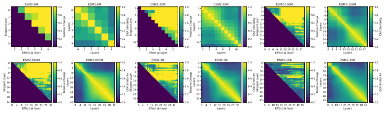
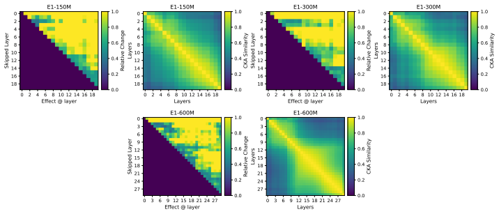
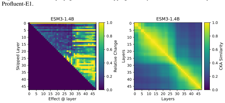
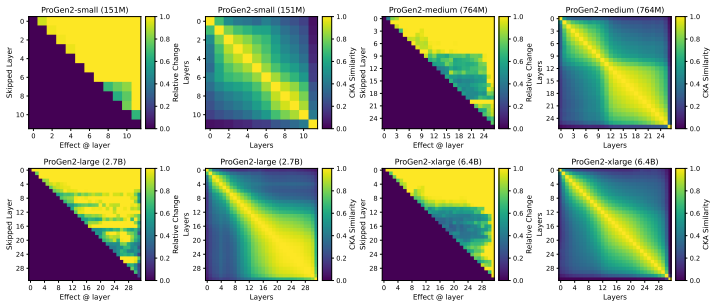
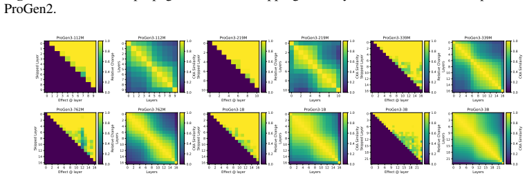
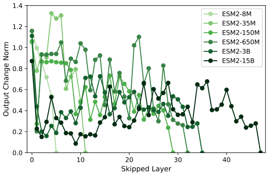
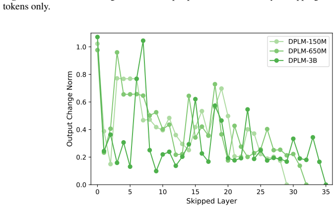
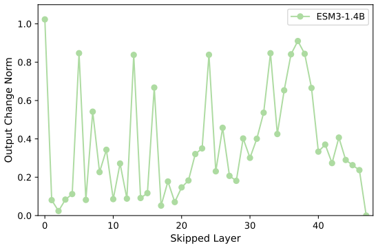
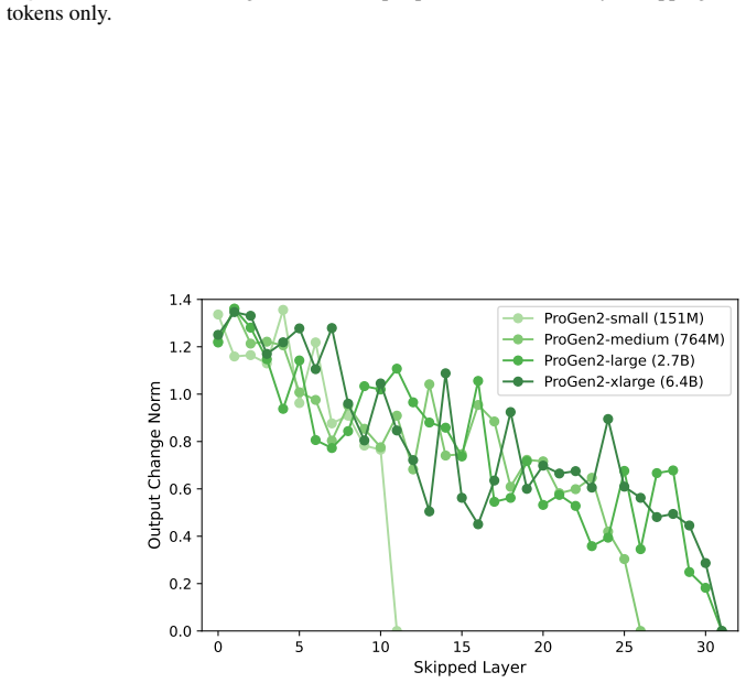
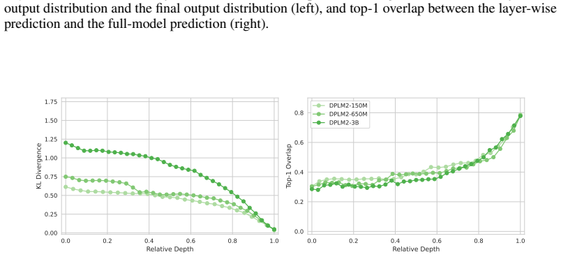
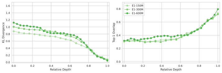
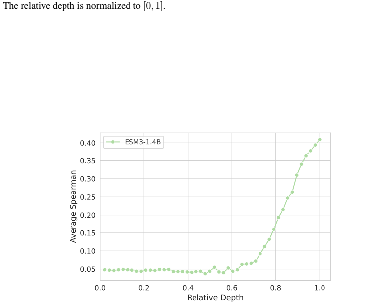
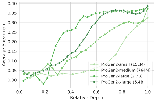
Across seven popular protein language model families spanning autoregressive, masked, and diffusion objectives at multiple scales, a large fraction of task-relevant computation is concentrated in a subset of layers, while the remaining layers mainly provide incremental refinement of the final prediction. These depth-dependent patterns persist beyond sequence-only settings and also appear in multimodal PLMs that accept both protein sequence and structure as input.

What carries the argument

A unified set of probing, perturbation, and downstream-evaluation measurements applied consistently across model families to quantify how each layer's contribution changes with depth.

If this is right

  • Many later layers can be removed or down-weighted with limited loss in task performance.
  • Training can be focused on strengthening the high-contribution layers rather than uniform depth scaling.
  • The same concentration pattern appears in both sequence-only and multimodal protein models.
  • Architectures that dynamically allocate computation to key layers may outperform fixed-depth transformers.

Where Pith is reading between the lines

These are editorial extensions of the paper, not claims the author makes directly.

  • Depth inefficiency may limit returns from simply making protein models deeper for tasks such as design or folding prediction.
  • Pruning or selective fine-tuning of the high-contribution layers could yield efficiency gains without retraining from scratch.
  • The pattern may extend to other biomolecular sequence models, suggesting a broader principle about how transformers process sequential biological data.

Load-bearing premise

The chosen probing, perturbation, and downstream measurements isolate each layer's actual contribution without being distorted by training objectives, architecture choices, or dataset properties.

What would settle it

A protein language model in which perturbing or probing any layer produces roughly equal performance drops on the same downstream tasks would show that computation is not concentrated in a subset of layers.

Figures

Figures reproduced from arXiv: 2602.21750 by Aleena Siji, Amir Mohammad Karimi Mamaghan, Andrea Dittadi, Emmanouil Angelis, Ferdinand Kapl, Johannes von Oswald, Kaitlin Maile, Karl Henrik Johansson, Maurice Brenner, Michael Heinzinger, Stefan Bauer, Tobias H\"oppe.

Figure 1
Figure 1. Figure 1: Maximum propagated effect of skipping each layer on future-token computations, [PITH_FULL_IMAGE:figures/full_fig_p005_1.png] view at source ↗
Figure 2
Figure 2. Figure 2: TunedLens analysis for ESM2 across depth: KL divergence to the final output [PITH_FULL_IMAGE:figures/full_fig_p006_2.png] view at source ↗
Figure 3
Figure 3. Figure 3: Layer-wise ProteinGym performance for ESM2. Average Spearman correlation as a function of relative depth, normalized to [0, 1], where predictions are taken from each layer. Per￾formance improves with depth for all model sizes, but the largest models exhibit diminishing returns in the final layers, suggesting that earlier layers already capture much of the signal and later layers mainly provide small refine… view at source ↗
Figure 4
Figure 4. Figure 4: Depth analysis results for ESM3 for the structure stream. [PITH_FULL_IMAGE:figures/full_fig_p008_4.png] view at source ↗
Figure 5
Figure 5. Figure 5: Cross-modal layer–layer co￾sine similarity between sequence-only and structure-only representations for ESM3. Each cell compares a sequence￾layer representation to a structure-layer representation for the same proteins, with similarities averaged across proteins. The first ∼60% of layers show high cross￾modal similarity, suggesting strong early sequence-structure alignment. After this point, similarity bec… view at source ↗
Figure 6
Figure 6. Figure 6: Maximum propagated effect of skipping each layer on future-token computations for DPLM. 0 3 6 9 12 15 18 21 24 27 Effect @ layer 0 3 6 9 12 15 18 21 24 27 Skipped Layer DPLM2-150M 0.0 0.2 0.4 0.6 0.8 1.0 Relative Change 0 3 6 9 12 15 18 21 24 27 Layers 0 3 6 9 12 15 18 21 24 27 Layers DPLM2-150M 0.0 0.2 0.4 0.6 0.8 1.0 CKA Similarity 0 4 8 12 16 20 24 28 32 Effect @ layer 0 4 8 12 16 20 24 28 32 Skipped La… view at source ↗
Figure 7
Figure 7. Figure 7: Maximum propagated effect of skipping each layer on future-token computations for DPLM2. B.2 How does the probability distribution vary across layers? Figures 19 to 24 report how the model’s token-level output distribution evolves across depth, using a layer-wise readout and comparing each layer’s distribution to the final-layer distribution. Lower KL divergence indicates that a layer already produces a di… view at source ↗
Figure 8
Figure 8. Figure 8: Maximum propagated effect of skipping each layer on future-token computations for Profluent-E1. 0 5 10 15 20 25 30 35 40 45 Effect @ layer 0 5 10 15 20 25 30 35 40 45 Skipped Layer ESM3-1.4B 0.0 0.2 0.4 0.6 0.8 1.0 Relative Change 0 5 10 15 20 25 30 35 40 45 Layers 0 5 10 15 20 25 30 35 40 45 Layers ESM3-1.4B 0.0 0.2 0.4 0.6 0.8 1.0 CKA Similarity [PITH_FULL_IMAGE:figures/full_fig_p018_8.png] view at source ↗
Figure 9
Figure 9. Figure 9: Maximum propagated effect of skipping each layer on later-layer representations (future tokens only), for ESM3. Overall, across all models, KL divergence generally decreases with depth and top-1 overlap increases, indicating that layer-wise predictions progressively align with the full-model output. For the largest variants in some families, these curves can become flat earlier in depth, suggesting that th… view at source ↗
Figure 10
Figure 10. Figure 10: Maximum propagated effect of skipping each layer on future-token computations for ProGen2. 0 1 2 3 4 5 6 7 8 9 Effect @ layer 0 1 2 3 4 5 6 7 8 9 Skipped Layer ProGen3-112M 0.0 0.2 0.4 0.6 0.8 1.0 Relative Change 0 1 2 3 4 5 6 7 8 9 Layers 0 1 2 3 4 5 6 7 8 9 Layers ProGen3-112M 0.0 0.2 0.4 0.6 0.8 1.0 CKA Similarity 0 2 4 6 8 10 Effect @ layer 0 2 4 6 8 10 Skipped Layer ProGen3-219M 0.0 0.2 0.4 0.6 0.8 1… view at source ↗
Figure 11
Figure 11. Figure 11: Maximum propagated effect of skipping each layer on future-token computations for ProGen3. B.3 How do different layers affect downstream performance? Figures 25 to 30 report layer-wise ProteinGym performance of the models, measured as average Spearman correlation as a function of relative depth (normalized to [0, 1]). These curves characterize where useful information for zero-shot fitness prediction is m… view at source ↗
Figure 12
Figure 12. Figure 12: Maximum change in ESM2 output probabilities under layer skipping, restricted to future tokens only. 0 5 10 15 20 25 30 35 Skipped Layer 0.0 0.2 0.4 0.6 0.8 1.0 Output Change Norm DPLM-150M DPLM-650M DPLM-3B [PITH_FULL_IMAGE:figures/full_fig_p020_12.png] view at source ↗
Figure 13
Figure 13. Figure 13: Maximum change in DPLM output probabilities under layer skipping, restricted to future tokens only. prediction head, so we use the same head in both settings. For ESM3, sequence and structure use separate prediction heads; accordingly, we use the structure head for the structure-only setting and the sequence head for the multimodal setting. Figures 39 and 42 show the structure-only analysis results for DP… view at source ↗
Figure 14
Figure 14. Figure 14: Maximum change in DPLM2 output probabilities under layer skipping, restricted to future tokens only. 0 5 10 15 20 25 30 Skipped Layer 0.0 0.2 0.4 0.6 0.8 1.0 1.2 Output Change Norm E1-150M E1-300M E1-600M [PITH_FULL_IMAGE:figures/full_fig_p021_14.png] view at source ↗
Figure 15
Figure 15. Figure 15: Maximum change in Profluent-E1 output probabilities under layer skipping, restricted to future tokens only. layer, and average the similarities across proteins [PITH_FULL_IMAGE:figures/full_fig_p021_15.png] view at source ↗
Figure 16
Figure 16. Figure 16: Maximum change in ESM3 output probabilities under layer skipping, restricted to future tokens only. 0 5 10 15 20 25 30 Skipped Layer 0.0 0.2 0.4 0.6 0.8 1.0 1.2 1.4 Output Change Norm ProGen2-small (151M) ProGen2-medium (764M) ProGen2-large (2.7B) ProGen2-xlarge (6.4B) [PITH_FULL_IMAGE:figures/full_fig_p022_16.png] view at source ↗
Figure 17
Figure 17. Figure 17: Maximum change in ProGen2 output probabilities under layer skipping, restricted to future tokens only. 22 [PITH_FULL_IMAGE:figures/full_fig_p022_17.png] view at source ↗
Figure 18
Figure 18. Figure 18: Maximum change in ProGen3 output probabilities under layer skipping, restricted to future tokens only. 0.0 0.2 0.4 0.6 0.8 1.0 Relative Depth 0.00 0.25 0.50 0.75 1.00 1.25 1.50 1.75 KL Divergence 0.0 0.2 0.4 0.6 0.8 1.0 Relative Depth 0.0 0.2 0.4 0.6 0.8 1.0 Top-1 Overlap DPLM-150M DPLM-650M DPLM-3B [PITH_FULL_IMAGE:figures/full_fig_p023_18.png] view at source ↗
Figure 19
Figure 19. Figure 19: TunedLens analysis for DPLM across depth: KL divergence between the layer-wise output distribution and the final output distribution (left), and top-1 overlap between the layer-wise prediction and the full-model prediction (right). 0.0 0.2 0.4 0.6 0.8 1.0 Relative Depth 0.00 0.25 0.50 0.75 1.00 1.25 1.50 1.75 KL Divergence 0.0 0.2 0.4 0.6 0.8 1.0 Relative Depth 0.0 0.2 0.4 0.6 0.8 Top-1 Overlap DPLM2-150M… view at source ↗
Figure 20
Figure 20. Figure 20: TunedLens analysis for DPLM2 across depth: KL divergence between the layer-wise output distribution and the final output distribution (left), and top-1 overlap between the layer-wise prediction and the full-model prediction (right). 23 [PITH_FULL_IMAGE:figures/full_fig_p023_20.png] view at source ↗
Figure 21
Figure 21. Figure 21: TunedLens analysis for E1 across depth: KL divergence between the layer-wise output distribution and the final output distribution (left), and top-1 overlap between the layer-wise prediction and the full-model prediction (right). 0.0 0.2 0.4 0.6 0.8 1.0 Relative Depth 0.0 0.2 0.4 0.6 0.8 1.0 1.2 1.4 KL Divergence 0.0 0.2 0.4 0.6 0.8 1.0 Relative Depth 0.0 0.2 0.4 0.6 0.8 Top-1 Overlap ESM3-1.4B [PITH_FUL… view at source ↗
Figure 22
Figure 22. Figure 22: TunedLens analysis for ESM3 across depth: KL divergence between the layer-wise output distribution and the final output distribution (left), and top-1 overlap between the layer-wise prediction and the full-model prediction (right). 0.0 0.2 0.4 0.6 0.8 1.0 Relative Depth 0.0 0.2 0.4 0.6 0.8 1.0 1.2 1.4 KL Divergence 0.0 0.2 0.4 0.6 0.8 1.0 Relative Depth 0.0 0.2 0.4 0.6 0.8 1.0 Top-1 Overlap ProGen2-small … view at source ↗
Figure 23
Figure 23. Figure 23: TunedLens analysis for ProGen2 across depth: KL divergence between the layer-wise output distribution and the final output distribution (left), and top-1 overlap between the layer-wise prediction and the full-model prediction (right). 24 [PITH_FULL_IMAGE:figures/full_fig_p024_23.png] view at source ↗
Figure 24
Figure 24. Figure 24: TunedLens analysis for ProGen3 across depth: KL divergence between the layer-wise output distribution and the final output distribution (left), and top-1 overlap between the layer-wise prediction and the full-model prediction (right). 0.0 0.2 0.4 0.6 0.8 1.0 Relative Depth 0.0 0.1 0.2 0.3 0.4 Average Spearman DPLM-150M DPLM-650M DPLM-3B [PITH_FULL_IMAGE:figures/full_fig_p025_24.png] view at source ↗
Figure 25
Figure 25. Figure 25: Average Spearman correlation for DPLM on ProteinGym, calculated at each layer. The relative depth is normalized to [0, 1]. 0.0 0.2 0.4 0.6 0.8 1.0 Relative Depth 0.0 0.1 0.2 0.3 0.4 Average Spearman DPLM2-150M DPLM2-650M DPLM2-3B [PITH_FULL_IMAGE:figures/full_fig_p025_25.png] view at source ↗
Figure 26
Figure 26. Figure 26: Average Spearman correlation for DPLM2 on ProteinGym, calculated at each layer. The relative depth is normalized to [0, 1]. 25 [PITH_FULL_IMAGE:figures/full_fig_p025_26.png] view at source ↗
Figure 27
Figure 27. Figure 27: Average Spearman correlation for Profluent-E1 on ProteinGym, calculated at each layer. The relative depth is normalized to [0, 1]. 0.0 0.2 0.4 0.6 0.8 1.0 Relative Depth 0.05 0.10 0.15 0.20 0.25 0.30 0.35 0.40 Average Spearman ESM3-1.4B [PITH_FULL_IMAGE:figures/full_fig_p026_27.png] view at source ↗
Figure 28
Figure 28. Figure 28: Average Spearman correlation for ESM3 on ProteinGym, calculated at each layer. The relative depth is normalized to [0, 1]. 26 [PITH_FULL_IMAGE:figures/full_fig_p026_28.png] view at source ↗
Figure 29
Figure 29. Figure 29: Average Spearman correlation for ProGen2 on ProteinGym, calculated at each layer. The relative depth is normalized to [0, 1]. 0.0 0.2 0.4 0.6 0.8 1.0 Relative Depth 0.0 0.1 0.2 0.3 0.4 Average Spearman ProGen3-112M ProGen3-219M ProGen3-339M ProGen3-762M ProGen3-1B ProGen3-3B [PITH_FULL_IMAGE:figures/full_fig_p027_29.png] view at source ↗
Figure 30
Figure 30. Figure 30: Average Spearman correlation for ProGen3 on ProteinGym, calculated at each layer. The relative depth is normalized to [0, 1]. 27 [PITH_FULL_IMAGE:figures/full_fig_p027_30.png] view at source ↗
Figure 31
Figure 31. Figure 31: Average Spearman correlation for ESM2 on ProteinGym, computed at each layer and shown separately by phenotype. Relative depth is normalized to [0, 1]. 28 [PITH_FULL_IMAGE:figures/full_fig_p028_31.png] view at source ↗
Figure 32
Figure 32. Figure 32: Average Spearman correlation for DPLM on ProteinGym, computed at each layer and shown separately by phenotype. Relative depth is normalized to [0, 1]. 29 [PITH_FULL_IMAGE:figures/full_fig_p029_32.png] view at source ↗
Figure 33
Figure 33. Figure 33: Average Spearman correlation for DPLM2 on ProteinGym, computed at each layer and shown separately by phenotype. Relative depth is normalized to [0, 1]. 30 [PITH_FULL_IMAGE:figures/full_fig_p030_33.png] view at source ↗
Figure 34
Figure 34. Figure 34: Average Spearman correlation for Profluent-E1 on ProteinGym, computed at each layer and shown separately by phenotype. Relative depth is normalized to [0, 1]. 31 [PITH_FULL_IMAGE:figures/full_fig_p031_34.png] view at source ↗
Figure 35
Figure 35. Figure 35: Average Spearman correlation for ESM3 on ProteinGym, computed at each layer and shown separately by phenotype. Relative depth is normalized to [0, 1]. 32 [PITH_FULL_IMAGE:figures/full_fig_p032_35.png] view at source ↗
Figure 36
Figure 36. Figure 36: Average Spearman correlation for ProGen2 on ProteinGym, computed at each layer and shown separately by phenotype. Relative depth is normalized to [0, 1]. 33 [PITH_FULL_IMAGE:figures/full_fig_p033_36.png] view at source ↗
Figure 37
Figure 37. Figure 37: Average Spearman correlation for ProGen3 on ProteinGym, computed at each layer and shown separately by phenotype. Relative depth is normalized to [0, 1]. 0 5 10 15 20 25 30 35 40 45 Effect @ layer 0 5 10 15 20 25 30 35 40 45 Skipped Layer ESM3-1.4B 0.0 0.2 0.4 0.6 0.8 1.0 Relative Change 0 5 10 15 20 25 30 35 40 45 Layers 0 5 10 15 20 25 30 35 40 45 Layers ESM3-1.4B 0.0 0.2 0.4 0.6 0.8 1.0 CKA Similarity … view at source ↗
Figure 38
Figure 38. Figure 38: Maximum propagated effect of skipping each layer on future-token computations of the multimodal (sequence-structure) stream for ESM3. 34 [PITH_FULL_IMAGE:figures/full_fig_p034_38.png] view at source ↗
Figure 39
Figure 39. Figure 39: Maximum propagated effect of skipping each layer on future-token computations of the structure stream for DPLM2. 0 3 6 9 12 15 18 21 24 27 Effect @ layer 0 3 6 9 12 15 18 21 24 27 Skipped Layer DPLM2-150M 0.0 0.2 0.4 0.6 0.8 1.0 Relative Change 0 3 6 9 12 15 18 21 24 27 Layers 0 3 6 9 12 15 18 21 24 27 Layers DPLM2-150M 0.0 0.2 0.4 0.6 0.8 1.0 CKA Similarity 0 4 8 12 16 20 24 28 32 Effect @ layer 0 4 8 12… view at source ↗
Figure 40
Figure 40. Figure 40: Maximum propagated effect of skipping each layer on future-token computations of the multimodal (sequence-structure) stream for DPLM2. 0.0 0.2 0.4 0.6 0.8 1.0 Relative Depth 0.0 0.5 1.0 1.5 2.0 2.5 3.0 3.5 4.0 KL Divergence 0.0 0.2 0.4 0.6 0.8 1.0 Relative Depth 0.0 0.2 0.4 0.6 0.8 Top-1 Overlap ESM3-1.4B [PITH_FULL_IMAGE:figures/full_fig_p035_40.png] view at source ↗
Figure 41
Figure 41. Figure 41: LogitLens analysis for ESM3 across depth on the multimodal (sequence-structure) stream: KL divergence between the layer-wise output distribution and the final output distribution (left), and top-1 overlap between the layer-wise prediction and the full-model prediction (right). 35 [PITH_FULL_IMAGE:figures/full_fig_p035_41.png] view at source ↗
Figure 42
Figure 42. Figure 42: LogitLens analysis for DPLM2 across depth on the structure stream: KL divergence between the layer-wise output distribution and the final output distribution (left), and top-1 overlap between the layer-wise prediction and the full-model prediction (right). 0.0 0.2 0.4 0.6 0.8 1.0 Relative Depth 0 2 4 6 8 10 KL Divergence 0.0 0.2 0.4 0.6 0.8 1.0 Relative Depth 0.0 0.1 0.2 0.3 0.4 0.5 0.6 0.7 0.8 Top-1 Over… view at source ↗
Figure 43
Figure 43. Figure 43: LogitLens analysis for DPLM2 across depth on the multimodal (sequence-structure) stream: KL divergence between the layer-wise output distribution and the final output distribution (left), and top-1 overlap between the layer-wise prediction and the full-model prediction (right). 0 3 6 9 12 15 18 21 24 27 Structure Layer 0 3 6 9 12 15 18 21 24 27 Sequence Layer DPLM2-150M 0.0 0.2 0.4 0.6 0.8 1.0 Cosine Simi… view at source ↗
Figure 44
Figure 44. Figure 44: Cross-modal layer–layer cosine similarity between sequence-only and structure-only representations for DPLM2, averaged across proteins. Each cell compares a sequence-layer represen￾tation to a structure-layer representation for the same proteins. 36 [PITH_FULL_IMAGE:figures/full_fig_p036_44.png] view at source ↗
read the original abstract

Protein language models (PLMs) have become widely adopted as general-purpose models, demonstrating strong performance in protein engineering and de novo design. Like large language models (LLMs), they are typically trained as deep transformers with next-token or masked-token prediction objectives on massive sequence corpora and are scaled by increasing model depth. Recent work on autoregressive LLMs has identified the Curse of Depth: many later layers contribute little to the final output predictions. These findings naturally raise the question of whether a similar depth inefficiency also appears in PLMs, where many widely used models are not autoregressive, and some are multimodal, accepting both protein sequence and structure as input. In this work, we present a depth analysis of seven popular PLM families across model scales, spanning autoregressive, masked, and diffusion objectives, and quantify how layer contributions evolve with depth using a unified set of probing-, perturbation-, and downstream-evaluation measurements. Across models, we observe consistent depth-dependent patterns that extend prior findings on LLMs: a large fraction of task-relevant computation is concentrated in a subset of layers, while the remaining layers mainly provide incremental refinement of the final prediction. These trends persist beyond sequence-only settings and also appear in multimodal PLMs. Taken together, our results suggest that depth inefficiency is a common feature of modern PLMs, motivating future work on more depth-efficient architectures and training methods.

Editorial analysis

A structured set of objections, weighed in public.

Desk editor's note, referee report, simulated authors' rebuttal, and a circularity audit. Tearing a paper down is the easy half of reading it; the pith above is the substance, this is the friction.

Referee Report

2 major / 1 minor

Summary. The manuscript investigates whether protein language models (PLMs) exhibit a 'curse of depth' analogous to that observed in large language models, wherein a large fraction of task-relevant computation concentrates in a subset of layers while others contribute mainly incremental refinement. Using a unified suite of probing, perturbation, and downstream-evaluation measurements, the authors analyze seven PLM families spanning autoregressive, masked, and diffusion objectives as well as multimodal (sequence+structure) variants, reporting consistent depth-dependent patterns that persist across model scales and input modalities.

Significance. If the central empirical patterns hold after addressing measurement validity, the work extends LLM depth analyses to the protein domain and supplies concrete motivation for depth-efficient PLM architectures, which would be valuable for protein engineering and design applications.

major comments (2)
  1. [Methods (perturbation experiments)] Methods (perturbation and probing sections): The headline claim that computation is concentrated in a subset of layers rests on the assumption that the chosen measurements cleanly isolate per-layer contributions. However, standard transformer residual connections allow early-layer activations to bypass later layers and reach the output head unchanged. No ablation that severs, re-scales, or compares against non-residual baselines is described, so the observed concentration could be an architectural artifact rather than evidence of depth inefficiency.
  2. [Results] Results (main figures and tables): The reported 'consistent patterns' are presented without error bars, confidence intervals, or statistical tests for cross-model agreement. This makes it difficult to evaluate the strength of the depth-dependent trends or to rule out that the patterns are driven by a few outlier models or tasks.
minor comments (1)
  1. [Abstract] Abstract: The phrase 'curse of depth' is used without a brief parenthetical reference to the specific prior LLM findings being extended, which would help readers unfamiliar with that literature.

Simulated Author's Rebuttal

2 responses · 0 unresolved

We thank the referee for the constructive feedback on measurement validity and statistical reporting. We address each major comment below and outline the revisions we will make to strengthen the manuscript.

read point-by-point responses
  1. Referee: [Methods (perturbation experiments)] Methods (perturbation and probing sections): The headline claim that computation is concentrated in a subset of layers rests on the assumption that the chosen measurements cleanly isolate per-layer contributions. However, standard transformer residual connections allow early-layer activations to bypass later layers and reach the output head unchanged. No ablation that severs, re-scales, or compares against non-residual baselines is described, so the observed concentration could be an architectural artifact rather than evidence of depth inefficiency.

    Authors: We appreciate this observation on residual connections. Our perturbation protocol intervenes on layer outputs (zeroing or scaling) while the residual pathways remain intact, so the measured change in final predictions or representations already reflects the incremental contribution of each layer atop the bypassed early activations. This is the standard way to quantify layer importance in residual transformers. We agree that a direct comparison to non-residual architectures would be informative, but it would require retraining multiple large models from scratch, which is outside the scope of the current study focused on existing PLMs. In the revision we will add an explicit paragraph in the Methods section describing how perturbations interact with residuals and include a small-scale controlled experiment on a non-residual toy transformer to illustrate the difference. revision: partial

  2. Referee: [Results] Results (main figures and tables): The reported 'consistent patterns' are presented without error bars, confidence intervals, or statistical tests for cross-model agreement. This makes it difficult to evaluate the strength of the depth-dependent trends or to rule out that the patterns are driven by a few outlier models or tasks.

    Authors: We agree that the absence of error bars and formal statistical tests weakens the presentation. In the revised manuscript we will recompute all main figures and tables with error bars (standard deviation across random seeds or data splits where applicable) and add statistical tests (Pearson correlation with depth, ANOVA across model families, and outlier-robustness checks) to quantify the consistency of the depth-dependent trends. These additions will be included in both the Results section and the supplementary material. revision: yes

Circularity Check

0 steps flagged

No significant circularity: purely empirical observational study

full rationale

The paper conducts a direct empirical analysis of seven existing public PLM families using standard probing, perturbation, and downstream metrics on pretrained models. No derivations, equations, fitted parameters renamed as predictions, or self-citation chains are used to support the central claims; observations are reported from measurements on off-the-shelf models without any self-referential construction or ansatz smuggling. The study is therefore self-contained against external benchmarks.

Axiom & Free-Parameter Ledger

0 free parameters · 1 axioms · 0 invented entities

No free parameters or invented entities; the work rests on standard domain assumptions about what probing and perturbation reveal in transformers.

axioms (1)
  • domain assumption Layer outputs can be meaningfully isolated and their contributions quantified via probing and perturbation without major confounding from residual connections or training dynamics.
    Invoked throughout the depth analysis methodology described in the abstract.

pith-pipeline@v0.9.0 · 5588 in / 1140 out tokens · 28570 ms · 2026-05-15T19:13:32.367674+00:00 · methodology

discussion (0)

Sign in with ORCID, Apple, or X to comment. Anyone can read and Pith papers without signing in.

Lean theorems connected to this paper

Citations machine-checked in the Pith Canon. Every link opens the source theorem in the public Lean library.

What do these tags mean?
matches
The paper's claim is directly supported by a theorem in the formal canon.
supports
The theorem supports part of the paper's argument, but the paper may add assumptions or extra steps.
extends
The paper goes beyond the formal theorem; the theorem is a base layer rather than the whole result.
uses
The paper appears to rely on the theorem as machinery.
contradicts
The paper's claim conflicts with a theorem or certificate in the canon.
unclear
Pith found a possible connection, but the passage is too broad, indirect, or ambiguous to say the theorem truly supports the claim.

Forward citations

Cited by 2 Pith papers

Reviewed papers in the Pith corpus that reference this work. Sorted by Pith novelty score.

  1. Layer Collapse in Diffusion Language Models

    cs.LG 2026-05 conditional novelty 7.0

    Early layers in diffusion language models like LLaDA-8B collapse into redundant representations around a critical super-outlier activation due to overtraining, making them more robust to quantization and sparsity than...

  2. Layer Collapse in Diffusion Language Models

    cs.LG 2026-05 unverdicted novelty 7.0

    Diffusion language models develop early-layer collapse around an indispensable super-outlier due to overtraining, resulting in higher compressibility and reversed optimal sparsity patterns versus autoregressive models.

Reference graph

Works this paper leans on

39 extracted references · 39 canonical work pages · cited by 1 Pith paper · 5 internal anchors

  1. [1]

    Eliciting Latent Predictions from Transformers with the Tuned Lens

    N. Belrose, Z. Furman, L. Smith, D. Halawi, I. Ostrovsky, L. McKinney, S. Biderman, and J. Steinhardt. Eliciting latent predictions from transformers with the tuned lens.arXiv preprint arXiv:2303.08112, 2023

  2. [2]

    Bhatnagar, S

    A. Bhatnagar, S. Jain, J. Beazer, S. C. Curran, A. M. Hoffnagle, K. S. Ching, M. Martyn, S. Nayfach, J. A. Ruffolo, and A. Madani. Scaling unlocks broader generation and deeper functional understanding of proteins.bioRxiv, pages 2025–04, 2025

  3. [3]

    Brandes, D

    N. Brandes, D. Ofer, Y . Peleg, N. Rappoport, and M. Linial. Proteinbert: a universal deep- learning model of protein sequence and function.Bioinformatics, 38(8):2102–2110, 2022

  4. [4]

    R. Chen, D. Xue, X. Zhou, Z. Zheng, Q. Gu, et al. An all-atom generative model for designing protein complexes. InF orty-second International Conference on Machine Learning, 2025

  5. [5]

    Y . Chen, J. Shang, Z. Zhang, Y . Xie, J. Sheng, T. Liu, S. Wang, Y . Sun, H. Wu, and H. Wang. Inner thinking transformer: Leveraging dynamic depth scaling to foster adaptive internal thinking.arXiv preprint arXiv:2502.13842, 2025

  6. [6]

    What Does BERT Look At? An Analysis of BERT's Attention

    K. Clark, U. Khandelwal, O. Levy, and C. D. Manning. What does bert look at? an analysis of bert’s attention.arXiv preprint arXiv:1906.04341, 2019

  7. [7]

    Csordás, C

    R. Csordás, C. D. Manning, and C. Potts. Do language models use their depth efficiently?arXiv preprint arXiv:2505.13898, 2025

  8. [8]

    Universal Transformers

    M. Dehghani, S. Gouws, O. Vinyals, J. Uszkoreit, and Ł. Kaiser. Universal transformers.arXiv preprint arXiv:1807.03819, 2018

  9. [9]

    Elnaggar, M

    A. Elnaggar, M. Heinzinger, C. Dallago, G. Rehawi, Y . Wang, L. Jones, T. Gibbs, T. Feher, C. Angerer, M. Steinegger, et al. Prottrans: Toward understanding the language of life through self-supervised learning.IEEE transactions on pattern analysis and machine intelligence, 44 (10):7112–7127, 2021

  10. [10]

    Ferruz, S

    N. Ferruz, S. Schmidt, and B. Höcker. Protgpt2 is a deep unsupervised language model for protein design.Nature communications, 13(1):4348, 2022

  11. [11]

    Geffner, K

    T. Geffner, K. Didi, Z. Cao, D. Reidenbach, Z. Zhang, C. Dallago, E. Kucukbenli, K. Kreis, and A. Vahdat. La-proteina: Atomistic protein generation via partially latent flow matching.arXiv preprint arXiv:2507.09466, 2025

  12. [12]

    Gromov, K

    A. Gromov, K. Tirumala, H. Shapourian, P. Glorioso, and D. Roberts. The unreasonable ineffectiveness of the deeper layers. InThe Thirteenth International Conference on Learning Representations, 2025

  13. [13]

    Hayes, R

    T. Hayes, R. Rao, H. Akin, N. J. Sofroniew, D. Oktay, Z. Lin, R. Verkuil, V . Q. Tran, J. Deaton, M. Wiggert, et al. Simulating 500 million years of evolution with a language model.Science, 387(6736):850–858, 2025

  14. [14]

    Hewitt and C

    J. Hewitt and C. D. Manning. A structural probe for finding syntax in word representations. InProceedings of the 2019 Conference of the North American Chapter of the Association for Computational Linguistics: Human Language Technologies, V olume 1 (Long and Short Papers), pages 4129–4138, 2019

  15. [15]

    S. Jain, J. Beazer, J. A. Ruffolo, A. Bhatnagar, and A. Madani. E1: Retrieval-augmented protein encoder models.bioRxiv, pages 2025–11, 2025

  16. [16]

    JUWELS Cluster and Booster: Exascale Pathfinder with Modular Supercomputing Architecture at Juelich Supercomputing Centre.Journal of large- scale research facilities, 7(A138), 2021

    Jülich Supercomputing Centre. JUWELS Cluster and Booster: Exascale Pathfinder with Modular Supercomputing Architecture at Juelich Supercomputing Centre.Journal of large- scale research facilities, 7(A138), 2021. doi: 10.17815/jlsrf-7-183. 11

  17. [17]

    F. Kapl, E. Angelis, T. Höppe, K. Maile, J. von Oswald, N. Scherrer, and S. Bauer. Do depth-grown models overcome the curse of depth? an in-depth analysis.arXiv preprint arXiv:2512.08819, 2025

  18. [18]

    F. Kapl, E. Angelis, K. Maile, J. von Oswald, and S. Bauer. From growing to looping: A unified view of iterative computation in llms.arXiv preprint arXiv:2602.16490, 2026

  19. [19]

    S. Karp, N. Saunshi, S. Miryoosefi, S. J. Reddi, and S. Kumar. Landscape-aware growing: The power of a little LAG.arXiv preprint arXiv:2406.02469, 2024

  20. [20]

    Kornblith, M

    S. Kornblith, M. Norouzi, H. Lee, and G. Hinton. Similarity of neural network representations revisited. InInternational conference on machine learning, pages 3519–3529. PMlR, 2019

  21. [21]

    V . Lad, J. H. Lee, W. Gurnee, and M. Tegmark. The remarkable robustness of LLMs: Stages of inference?arXiv preprint arXiv:2406.19384, 2024

  22. [22]

    Z. Lin, H. Akin, R. Rao, B. Hie, Z. Zhu, W. Lu, N. Smetanin, R. Verkuil, O. Kabeli, Y . Shmueli, et al. Evolutionary-scale prediction of atomic-level protein structure with a language model. Science, 379(6637):1123–1130, 2023

  23. [23]

    Madani, B

    A. Madani, B. McCann, N. Naik, N. S. Keskar, N. Anand, R. R. Eguchi, P.-S. Huang, and R. Socher. Progen: Language modeling for protein generation.arXiv preprint arXiv:2004.03497, 2020

  24. [24]

    Meier, R

    J. Meier, R. Rao, R. Verkuil, J. Liu, T. Sercu, and A. Rives. Language models enable zero-shot prediction of the effects of mutations on protein function.Advances in Neural Information Processing Systems, 34:29287–29303, 2021

  25. [25]

    Muhtar, X

    D. Muhtar, X. Song, S. Pokutta, M. Zimmer, N. Pelleriti, T. Hofmann, and S. Liu. When does sparsity mitigate the curse of depth in llms.arXiv preprint arXiv:2603.15389, 2026

  26. [26]

    Nijkamp, J

    E. Nijkamp, J. A. Ruffolo, E. N. Weinstein, N. Naik, and A. Madani. Progen2: exploring the boundaries of protein language models.Cell systems, 14(11):968–978, 2023

  27. [27]

    Interpreting GPT: The logit lens, 2020

    Nostalgebraist. Interpreting GPT: The logit lens, 2020. URL https://www.lesswrong.com/ posts/AcKRB8wDpdaN6v6ru/interpreting-gpt-the-logit-lens

  28. [28]

    Notin, A

    P. Notin, A. Kollasch, D. Ritter, L. Van Niekerk, S. Paul, H. Spinner, N. Rollins, A. Shaw, R. Orenbuch, R. Weitzman, et al. Proteingym: Large-scale benchmarks for protein fitness prediction and design.Advances in Neural Information Processing Systems, 36:64331–64379, 2023

  29. [29]

    R. Rao, N. Bhattacharya, N. Thomas, Y . Duan, P. Chen, J. Canny, P. Abbeel, and Y . Song. Evaluating protein transfer learning with tape.Advances in Neural Information Processing Systems, 32, 2019

  30. [30]

    Rives, J

    A. Rives, J. Meier, T. Sercu, S. Goyal, Z. Lin, J. Liu, D. Guo, M. Ott, C. L. Zitnick, J. Ma, et al. Biological structure and function emerge from scaling unsupervised learning to 250 million protein sequences.Proceedings of the National Academy of Sciences, 118(15):e2016239118, 2021

  31. [31]

    Saunshi, S

    N. Saunshi, S. Karp, S. Krishnan, S. Miryoosefi, S. Jakkam Reddi, and S. Kumar. On the inductive bias of stacking towards improving reasoning.Advances in Neural Information Processing Systems, 37:71437–71464, 2024

  32. [32]

    Layer by Layer: Uncovering Hidden Representations in Language Models

    O. Skean, M. R. Arefin, D. Zhao, N. Patel, J. Naghiyev, Y . LeCun, and R. Shwartz-Ziv. Layer by layer: Uncovering hidden representations in language models.arXiv preprint arXiv:2502.02013, 2025

  33. [33]

    W. Sun, X. Song, P. Li, L. Yin, Y . Zheng, and S. Liu. The curse of depth in large language models.arXiv preprint arXiv:2502.05795, 2025

  34. [34]

    B. E. Suzek, H. Huang, P. McGarvey, R. Mazumder, and C. H. Wu. Uniref: comprehensive and non-redundant uniprot reference clusters.Bioinformatics, 23(10):1282–1288, 2007. 12

  35. [35]

    What do you learn from context? Probing for sentence structure in contextualized word representations

    I. Tenney, P. Xia, B. Chen, A. Wang, A. Poliak, R. T. McCoy, N. Kim, B. Van Durme, S. R. Bowman, D. Das, et al. What do you learn from context? probing for sentence structure in contextualized word representations.arXiv preprint arXiv:1905.06316, 2019

  36. [36]

    Vaswani, N

    A. Vaswani, N. Shazeer, N. Parmar, J. Uszkoreit, L. Jones, A. N. Gomez, Ł. Kaiser, and I. Polosukhin. Attention is all you need.Advances in Neural Information Processing Systems, 30, 2017

  37. [37]

    X. Wang, Z. Zheng, F. Ye, D. Xue, S. Huang, and Q. Gu. Diffusion language models are versatile protein learners. InInternational Conference on Machine Learning, pages 52309–52333. PMLR, 2024

  38. [38]

    X. Wang, Z. Zheng, D. Xue, S. Huang, Q. Gu, et al. Dplm-2: A multimodal diffusion protein language model. InThe Thirteenth International Conference on Learning Representations, 2025

  39. [39]

    J. Wei, X. Wang, D. Schuurmans, M. Bosma, F. Xia, E. Chi, Q. V . Le, D. Zhou, et al. Chain-of- thought prompting elicits reasoning in large language models.Advances in Neural Information Processing Systems, 35:24824–24837, 2022. 13 A Experimental Details In this section, we explain the included PLMs and provide full details of the experiments used in our ...