From One-Pass SGD to Data Reuse: Mini-Batch Scaling Laws in Sketched Linear Regression
Pith reviewed 2026-06-30 14:05 UTC · model grok-4.3
The pith
Mini-batching preserves bias exponents in sketched linear regression but scales variance as O(min(M,(T_eff γ)^{1/a})/(B T_eff)) for one-pass SGD while only changing fluctuation covariance for multi-pass methods.
A machine-rendered reading of the paper's core claim, the machinery that carries it, and where it could break.
Core claim
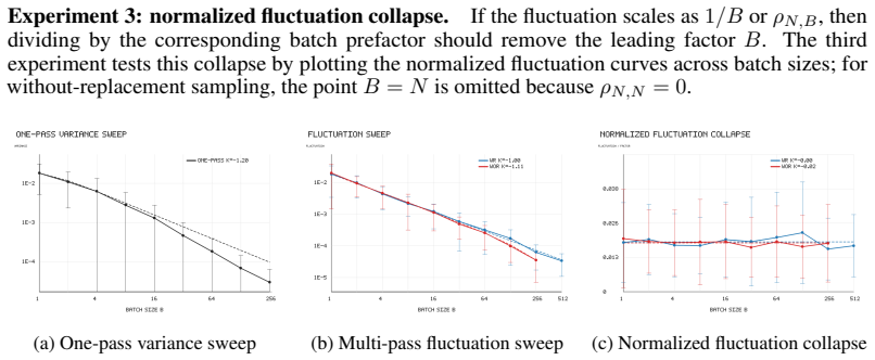
Under a power-law covariance spectrum and source condition the paper proves that one-pass batch SGD variance scales as O(min(M,(T_eff γ)^{1/a})/(B T_eff)), preserving approximation and optimization-bias exponents, while the two multi-pass batch SGD variants share approximation, GD bias and GD variance terms and differ only in the fluctuation covariance prefactor (1/B with replacement, ho_{N,B} without replacement). When B=N the fluctuation term vanishes and deterministic gradient descent is recovered.
What carries the argument
Risk decomposition separating shared approximation/GD bias/variance terms from protocol-dependent stochastic terms, analyzed under power-law spectrum and source condition to obtain explicit scaling exponents in batch size B, effective iterations T_eff and dimension M.
If this is right
- Mini-batching preserves approximation and optimization-bias exponents in one-pass SGD.
- At fixed update count T the 1/B variance reduction holds, but in the one-pass regime T=N/B this reduction is partly offset by the shorter optimization horizon.
- Multi-pass with- and without-replacement sampling share approximation and GD bias/variance terms exactly.
- Without-replacement sampling yields lower fluctuation covariance than with-replacement for B>1, and the fluctuation term vanishes at B=N recovering deterministic GD.
Where Pith is reading between the lines
- The decomposition suggests batch size can be traded directly against total data volume when optimizing total compute in one-pass regimes.
- Similar source-condition scaling may appear in non-linear models if their effective spectra remain approximately power-law after sketching.
- Without-replacement sampling could support larger practical batch sizes before noise increases, provided the ho_{N,B} formula continues to govern fluctuation.
- The results place batch size on equal footing with model dimension and data volume in compute-optimal scaling arguments for linear sketched problems.
Load-bearing premise
The derivations rely on a power-law covariance spectrum together with a source condition on the target parameter; if these spectral assumptions fail to hold for the data, the claimed exponents and min-function scaling no longer apply.
What would settle it
Observe whether empirical variance of one-pass mini-batch SGD on a dataset with non-power-law covariance eigenvalues follows the predicted O(min(M,(T_eff γ)^{1/a})/(B T_eff)) form as B and T_eff vary.
Figures
read the original abstract
Scaling laws provide compact descriptions of how prediction error varies with compute, model size, and data, but existing theory mainly treats single-sample SGD or full data reuse, leaving the role of mini-batching unclear. We study batch scaling laws for sketched linear regression under a power-law covariance spectrum and a source condition on the target parameter. We analyze one-pass batch SGD, multi-pass batch SGD with replacement, and multi-pass batch SGD without replacement. Our first result is a risk decomposition: all three procedures share the same irreducible and approximation terms, while their stochastic terms depend on the sampling protocol. One-pass batch SGD splits into bias and variance, whereas the two multi-pass methods split into GD bias, GD variance, and a fluctuation term around a common GD reference trajectory. We then prove source-condition scaling laws for one-pass and multi-pass mini-batch methods. For one-pass batch SGD, mini-batching preserves the approximation and optimization-bias exponents, while the variance scales as $O(\min(M,(T_{\mathrm{eff}}\gamma)^{1/a})/(B T_{\mathrm{eff}}))$. Thus the usual $1/B$ covariance reduction holds at fixed update count $T$, but in the one-pass regime $T=N/B$ it is partly offset by the shorter optimization horizon. For multi-pass batch SGD, with- and without-replacement sampling have identical approximation and GD bias/variance terms; they differ only in the fluctuation covariance prefactor, which is $1/B$ with replacement and $\rho_{N,B}=(N-B)/(B(N-1))$ without replacement. Hence without-replacement sampling is less noisy for $B>1$, and when $B=N$ the fluctuation vanishes, recovering deterministic gradient descent. These results place batch size on the same theoretical footing as compute, data, and model dimension in sketched linear regression.
Editorial analysis
A structured set of objections, weighed in public.
Referee Report
Summary. The paper derives a risk decomposition for sketched linear regression under mini-batch SGD variants (one-pass batch SGD, multi-pass with replacement, multi-pass without replacement) assuming a power-law covariance spectrum λ_j ∼ j^{-a} and source condition on θ^*. All protocols share irreducible and approximation terms; one-pass splits into bias/variance while multi-pass splits into GD bias/variance plus fluctuation. It proves scaling laws in which one-pass variance is O(min(M, (T_eff γ)^{1/a})/(B T_eff)), multi-pass protocols share GD terms and differ only in fluctuation prefactor (1/B vs. ρ_{N,B}=(N-B)/(B(N-1))), and concludes that batch size B stands on equal footing with compute, data, and dimension.
Significance. If the derivations hold, the explicit risk decomposition and closed-form scaling expressions under the stated spectral assumptions provide a useful theoretical tool for incorporating mini-batching into scaling-law analyses of linear models. The clean separation of terms and the recovery of deterministic GD at B=N are strengths. The work is appropriately conditional on the power-law spectrum and source condition; this does not undermine the internal claims but limits direct extrapolation beyond that regime.
major comments (2)
- [§3] §3 (risk decomposition): the claim that irreducible and approximation terms are identical across all three protocols is load-bearing for the later scaling comparisons. The derivation must explicitly verify that the source-condition parameter β enters these terms uniformly and independently of the sampling protocol (with/without replacement or one-pass), otherwise the separation into 'shared' vs. 'protocol-dependent stochastic' terms does not hold.
- [§5] §5 (one-pass scaling laws), variance expression: the O(min(M,(T_eff γ)^{1/a})/(B T_eff)) form is obtained after invoking the power-law spectrum to define both M and the exponent 1/a. The proof must confirm that the fluctuation-term analysis introduces no additional B-dependent factors that would alter the min expression or the claimed 1/B covariance reduction at fixed T; otherwise the 'batch size on the same footing' conclusion is not supported at the stated level of generality.
minor comments (2)
- The effective quantities T_eff, γ, and M are used throughout the scaling statements but their precise definitions (in terms of N, B, a, β) should be recalled once in the introduction or abstract for self-contained reading.
- Notation for the covariance operator eigenvalues and the source-condition norm should be introduced before the first use of the scaling expressions to avoid forward references.
Simulated Author's Rebuttal
We thank the referee for the thorough review and the recommendation for minor revision. The comments help clarify the presentation of our results. We address each major comment below.
read point-by-point responses
-
Referee: [§3] §3 (risk decomposition): the claim that irreducible and approximation terms are identical across all three protocols is load-bearing for the later scaling comparisons. The derivation must explicitly verify that the source-condition parameter β enters these terms uniformly and independently of the sampling protocol (with/without replacement or one-pass), otherwise the separation into 'shared' vs. 'protocol-dependent stochastic' terms does not hold.
Authors: We thank the referee for this observation. In the derivation of the risk decomposition in Section 3, the irreducible term is the variance of the additive noise in the labels, which is independent of the sampling protocol by construction. The approximation term is determined by the tail of the spectrum beyond the effective dimension and the source condition parameter β, which governs the decay of the coefficients of θ^* in the eigenbasis. Since this term is computed from the population quantities (the covariance operator and θ^*) without reference to the stochastic sampling process, it is identical for all protocols. The protocol dependence appears only in the stochastic terms (variance for one-pass, GD variance and fluctuation for multi-pass). To make this explicit, we will add a clarifying sentence in §3. revision: partial
-
Referee: [§5] §5 (one-pass scaling laws), variance expression: the O(min(M,(T_eff γ)^{1/a})/(B T_eff)) form is obtained after invoking the power-law spectrum to define both M and the exponent 1/a. The proof must confirm that the fluctuation-term analysis introduces no additional B-dependent factors that would alter the min expression or the claimed 1/B covariance reduction at fixed T; otherwise the 'batch size on the same footing' conclusion is not supported at the stated level of generality.
Authors: In the proof for the one-pass case in §5, the variance term is analyzed directly from the covariance of the mini-batch gradient estimator. Under the assumption of sampling without replacement within the batch or with large data, the covariance is exactly (1/B) times the single-sample covariance. The power-law spectrum is used to bound the trace or the effective rank M, leading to the min(M, ...) expression, but this bound does not introduce extra B-dependent factors in the scaling; the 1/B is preserved. The fluctuation term mentioned is for the multi-pass protocols and is analyzed separately. The conclusion that batch size is on equal footing follows from this 1/B factor at fixed T_eff. We believe the existing proof already confirms this, so no revision is required. revision: no
Circularity Check
No circularity; scaling laws are direct mathematical consequences of explicitly stated power-law spectrum and source condition
full rationale
The paper declares upfront that all results hold under the assumptions of a power-law covariance spectrum λ_j ∼ j^{-a} together with a source condition on θ^*. The risk decomposition, one-pass variance bound O(min(M,(T_eff γ)^{1/a})/(B T_eff)), and the separation into approximation/GD-bias/fluctuation terms are then proved as consequences of these spectral assumptions. No prediction is obtained by fitting a parameter to data inside the paper and then relabeling it; no load-bearing step reduces to a self-citation whose content is itself unverified; and the functional forms (including the min expression and the ρ_{N,B} prefactor) are fixed by the external assumptions rather than by internal redefinition. The derivation chain is therefore self-contained.
Axiom & Free-Parameter Ledger
free parameters (2)
- power-law exponent a
- source condition parameter
axioms (2)
- domain assumption Power-law covariance spectrum
- domain assumption Source condition on target parameter
Forward citations
Cited by 1 Pith paper
-
Sketched Linear Contrastive Learning: Approximation, Optimization, and Statistical Scaling
Derives explicit scaling law for risk in sketched linear contrastive learning w.r.t. sketch dimension M, sample size N, and optimization horizon under paired Gaussian and power-law assumptions.
Reference graph
Works this paper leans on
-
[1]
Scaling and renormalization in high-dimensional regression
Alexander Atanasov, Jacob A. Zavatone-Veth, and Cengiz Pehlevan. Scaling and renormalization in high-dimensional regression.arXiv preprint arXiv:2405.00592,
work page internal anchor Pith review Pith/arXiv arXiv
-
[2]
Chinchilla scaling: A replication attempt.arXiv preprint arXiv:2404.10102,
Tamay Besiroglu, Ege Erdil, Matthew Barnett, and Josh You. Chinchilla scaling: A replication attempt.arXiv preprint arXiv:2404.10102,
-
[3]
Accurate, Large Minibatch SGD: Training ImageNet in 1 Hour
Priya Goyal, Piotr Dollár, Ross Girshick, Pieter Noordhuis, Lukasz Wesolowski, Aapo Kyrola, Andrew Tulloch, Yangqing Jia, and Kaiming He. Accurate, large minibatch SGD: Training ImageNet in 1 hour.arXiv preprint arXiv:1706.02677,
work page internal anchor Pith review Pith/arXiv arXiv
-
[4]
Scaling Laws for Autoregressive Generative Modeling
Tom Henighan, Jared Kaplan, Mor Katz, Mark Chen, Christopher Hesse, Jacob Jackson, Heewoo Jun, Tom B. Brown, Prafulla Dhariwal, Scott Gray, Chris Hallacy, Ben Mann, Alec Radford, Aditya Ramesh, Daniel M. Ziegler, Dario Amodei, and Sam McCandlish. Scaling laws for autoregressive generative modeling.arXiv preprint arXiv:2010.14701,
work page internal anchor Pith review Pith/arXiv arXiv 2010
-
[5]
Deep Learning Scaling is Predictable, Empirically
Joel Hestness, Sharan Narang, Newsha Ardalani, Gregory Diamos, Heewoo Jun, Hassan Kianinejad, Md. Mostofa Ali Patwary, Yang Yang, and Yanqi Zhou. Deep learning scaling is predictable, empirically.arXiv preprint arXiv:1712.00409,
work page internal anchor Pith review Pith/arXiv arXiv
-
[6]
Hutter, Learning curve theory, arXiv preprint arXiv:2102.04074 (2021)
Marcus Hutter. Learning curve theory.arXiv preprint arXiv:2102.04074,
-
[7]
Scaling Laws for Neural Language Models
Jared Kaplan, Sam McCandlish, Tom Henighan, Tom B. Brown, Benjamin Chess, Rewon Child, Scott Gray, Alec Radford, Jeffrey Wu, and Dario Amodei. Scaling laws for neural language models. arXiv preprint arXiv:2001.08361,
work page internal anchor Pith review Pith/arXiv arXiv 2001
-
[8]
Alexander Maloney, Daniel A. Roberts, and James Sully. A solvable model of neural scaling laws. arXiv preprint arXiv:2210.16859,
-
[9]
An Empirical Model of Large-Batch Training
Sam McCandlish, Jared Kaplan, Dario Amodei, and OpenAI Team. An empirical model of large-batch training.arXiv preprint arXiv:1812.06162,
work page internal anchor Pith review Pith/arXiv arXiv
-
[10]
A neural scaling law from the dimension of the data manifold
Utkarsh Sharma and Jared Kaplan. A neural scaling law from the dimension of the data manifold. arXiv preprint arXiv:2004.10802,
-
[11]
Scaling law for language models training considering batch size.arXiv preprint arXiv:2412.01505,
Xian Shuai, Yiding Wang, Yimeng Wu, Xin Jiang, and Xiaozhe Ren. Scaling law for language models training considering batch size.arXiv preprint arXiv:2412.01505,
-
[12]
Large Batch Training of Convolutional Networks
Yang You, Igor Gitman, and Boris Ginsburg. Large batch training of convolutional networks.arXiv preprint arXiv:1708.03888,
work page internal anchor Pith review Pith/arXiv arXiv
-
[13]
14 A.2 Notations and setup formulas for normal GD
12 From One-Pass SGD to Data Reuse: Mini-Batch Scaling Laws in Sketched Linear Regression Supplementary Material Table of Contents A Appendix Preliminaries 14 A.1 Block notation . . . . . . . . . . . . . . . . . . . . . . . . . . . . . . . . . . . . . . . . . . . . . . . . . 14 A.2 Notations and setup formulas for normal GD . . . . . . . . . . . . . . . ....
2024
-
[14]
Step 1 gives Ebatch[ξ(B) t ] = 0, and taking expectation over the batch randomness in equation 24 gives the covariance part of assump- tion(2)with σ2 ξ = σ2 ξ,B B
Moreover, since θt−1 is deterministic once (S, w∗, D) are fixed and each mini-batch is sampled inde- pendently across iterations, the pair(At, ξ(B) t ) is independent of Ft−1. Step 1 gives Ebatch[ξ(B) t ] = 0, and taking expectation over the batch randomness in equation 24 gives the covariance part of assump- tion(2)with σ2 ξ = σ2 ξ,B B . Therefore, using...
2025
-
[15]
Let ε∈(0,1) , and suppose in addition that Leff ≲N (1−ε)a/γ. Then there exists an(a, ε)-dependent constantc >0such that, whenever γ≤ c logN , we have with probability at least 1−exp(−Ω(M)) over the randomness ofS, E[Flucwr B ]≲ γlogN B (Leffγ)1/a−1 + (Leffγ)1/a N . Proof. We imitate the Gaussian concentration estimates and leave-one-out argument as in Ap-...
2025
-
[16]
random PSD matrices over the batch randomness, and Ebatch[At] = Σν,E batch[A2 t ]⪯C AΣν,∥Σ ν∥2 ≤C A
Then(A t)t∈[L] are i.i.d. random PSD matrices over the batch randomness, and Ebatch[At] = Σν,E batch[A2 t ]⪯C AΣν,∥Σ ν∥2 ≤C A. Moreover, if γ0 := min 1 8CA , γ , then γ0CA ≤1/8 , hence 4γ0CA ≤1/2<1 . In particular, these are exactly the mean and matrix-moment bounds needed later to apply Lemma I.4 withA t =bΣ(B) t andΣ ν =bΣ. 46 Proof.Write zi :=Sx i, Z i...
2025
-
[17]
and Sections A and G of Lin et al. [2024]. These are the spectral, moment, and concentration ingredients used repeatedly across the appendix proofs for equation 2, equation 3, and equation
2024
discussion (0)
Sign in with ORCID, Apple, or X to comment. Anyone can read and Pith papers without signing in.