Optimal classical shadow estimation of unitary channels at Heisenberg limit
Pith reviewed 2026-06-27 06:20 UTC · model grok-4.3
The pith
A parallel non-adaptive protocol estimates expectation values of unitary channels to error ε with O(d ε^{-1}) queries when states or observables have constant rank and matches a proven lower bound.
A machine-rendered reading of the paper's core claim, the machinery that carries it, and where it could break.
Core claim
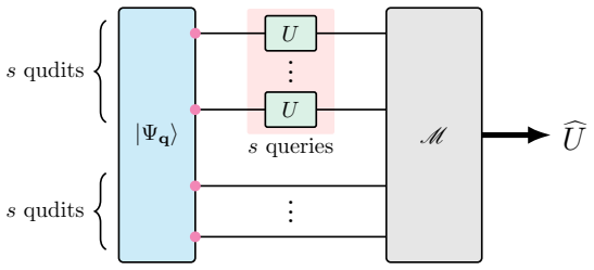
The central claim is that there exists a parallel, non-adaptive protocol for classical shadow estimation of unitary channels (CSEU) that uses O(d ε^{-1}) queries to achieve additive error ε whenever the input states or observables have constant rank, together with a matching Ω(d ε^{-1}) lower bound that remains valid under stronger access models; this protocol is then used to obtain optimal parallel-query solutions for unitary channel tomography and several other quantum learning tasks.
What carries the argument
The parallel non-adaptive CSEU protocol that converts queries to the unknown unitary into classical shadow data for later prediction of expectation values.
If this is right
- Optimal unitary channel tomography is possible with only parallel queries, closing the previous gap with sequential protocols.
- Hamiltonian learning, Pauli transfer matrix learning, and inverse-free amplitude estimation inherit the same O(d ε^{-1}) query bound under constant-rank conditions.
- Boundary-regime quantum channel tomography and shallow-circuit learning obtain improved query complexity via the same CSEU construction.
- Pure-state property estimation tasks can be reduced to the CSEU setting with the stated scaling.
Where Pith is reading between the lines
- The constant-rank restriction may be removable in future work by combining the protocol with rank-reduction preprocessing steps.
- The parallel-query optimality result suggests that many other quantum process learning problems previously thought to require adaptivity can be solved non-adaptively at the same cost.
- Experimental implementations on near-term devices could test the protocol by verifying Heisenberg scaling on small constant-rank observables before scaling to larger systems.
Load-bearing premise
The stated query scaling holds only when the input states or observables have constant rank.
What would settle it
An explicit family of constant-rank states and observables together with a unitary channel for which no parallel protocol with o(d ε^{-1}) queries can achieve error ε would falsify the claimed optimality.
Figures


read the original abstract
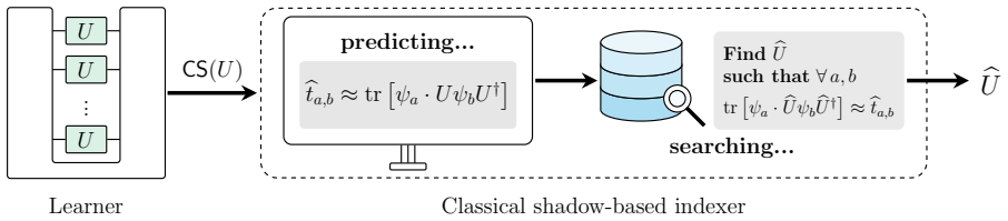
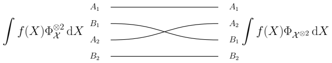
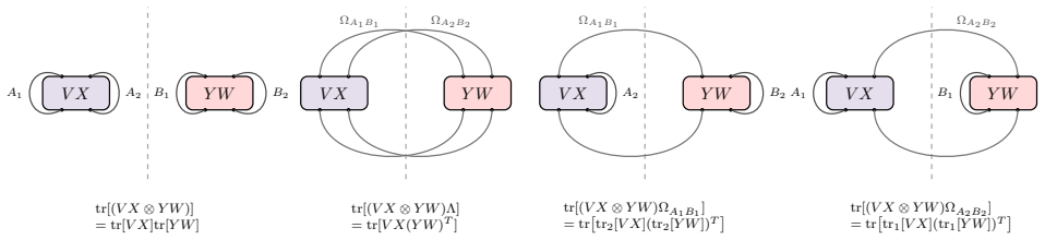
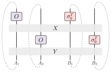
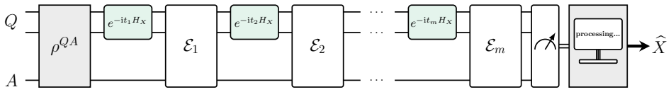
Full tomography of an unknown quantum evolution is resource-intensive and often unnecessary when the goal is only to predict selected properties. This motivates the study of classical shadow estimation of unitary channels (CSEU), a task in which one queries an unknown $d$-dimensional unitary $U$ and stores classical data that can later be used to predict expectation values $\mathrm{tr}[O \cdot U\rho U^\dagger]$ up to additive error $\varepsilon$ for arbitrary input states $\rho$ and observables $O$. We propose a parallel, non-adaptive CSEU protocol using $\mathcal{O}(d\varepsilon^{-1})$ queries when the input states or observables have constant rank. This achieves Heisenberg scaling with respect to $\varepsilon$ and is query-optimal, as we prove a matching $\Omega(d\varepsilon^{-1})$ lower bound that remains valid even with stronger access to the unknown unitary. Our query-optimal CSEU protocol provides a versatile and powerful tool for quantum learning theory, pushing the performance limits of several fundamental learning tasks, including unitary channel tomography, Hamiltonian learning, boundary-regime quantum channel tomography, Pauli transfer matrix learning, inverse-free amplitude estimation, pure-state property estimation, and shallow-circuit learning. Remarkably, we show that optimal unitary channel tomography can be achieved using only parallel queries, closing the gap between the best achievable efficiency of parallel and sequential tomography protocols. Together, these applications establish our framework as a fundamental tool for learning properties of quantum processes, particularly for certain key tasks that require high precision.
Editorial analysis
A structured set of objections, weighed in public.
Referee Report
Summary. The paper proposes a parallel, non-adaptive protocol for classical shadow estimation of unitary channels (CSEU) that uses O(d ε^{-1}) queries to predict tr[O U ρ U†] to additive error ε when the input state ρ or observable O has constant rank. It claims this achieves Heisenberg scaling in ε and proves a matching Ω(d ε^{-1}) lower bound that holds even under stronger access models to the unknown unitary U. The framework is then applied to improve query complexity for tasks including unitary channel tomography (achieving optimality with only parallel queries), Hamiltonian learning, Pauli transfer matrix learning, and others.
Significance. If the protocol construction and lower bound are correct, the result is significant for quantum learning theory: it supplies a query-optimal, parallel CSEU primitive under the constant-rank restriction and demonstrates that parallel queries suffice for optimal unitary tomography, closing a gap with sequential protocols. The applications to multiple learning tasks further indicate broad utility when the rank condition is met.
minor comments (2)
- [Abstract / lower-bound section] The abstract states the lower bound 'remains valid even with stronger access,' but the manuscript should explicitly identify the stronger access model (e.g., in the lower-bound section) and confirm that the constant-rank assumption is used symmetrically in both upper and lower bounds.
- Notation for the constant-rank condition (e.g., how 'constant rank' is formalized with respect to d) should be introduced early and used consistently when stating the O(d ε^{-1}) and Ω(d ε^{-1}) scalings.
Simulated Author's Rebuttal
We thank the referee for the positive assessment of our work on optimal parallel CSEU and the recommendation for minor revision. The report correctly identifies the key contributions, including the O(d ε^{-1}) query complexity, Heisenberg scaling, and the matching lower bound under stronger access models, as well as the applications to tomography and other tasks.
Circularity Check
No significant circularity; derivation self-contained under stated assumptions
full rationale
The paper explicitly conditions both the O(d ε^{-1}) protocol and the matching Ω(d ε^{-1}) lower bound on the constant-rank assumption for ρ or O, presents the lower bound as holding under stronger access models, and offers no self-citations, fitted parameters renamed as predictions, or self-definitional steps in the provided abstract and claims. The optimality result is therefore a conditional theorem whose proof chain does not reduce to its own inputs by construction.
Axiom & Free-Parameter Ledger
axioms (1)
- standard math Standard framework of quantum mechanics including unitary operators, density matrices, and trace-based expectation values.
Forward citations
Cited by 1 Pith paper
-
Near-Optimal Learning of Local Lindbladians
Near-optimal algorithm learns local Lindbladians via finite-time probes and classical shadows with Õ(Λ²/ε²) channel uses and matching lower bounds showing dissipative terms block Heisenberg-limited scaling.
Reference graph
Works this paper leans on
-
[1]
3 [ADOY25] Anurag Anshu, Yangjing Dong, Fengning Ou, and Penghui Yao
Association for Computing Machinery. 3 [ADOY25] Anurag Anshu, Yangjing Dong, Fengning Ou, and Penghui Yao. On the computational power of QAC0 with barely superlinear ancillae. InProceedings of the 57th Annual ACM Symposium on Theory of Computing, STOC ’25, page 1476–1487, New York, NY, USA, 2025. Association for Computing Machinery. 18 [Ang25] Armando Ang...
2025
-
[2]
American Mathematical Society, August 2017
3 [AS17] Guillaume Aubrun and Stanisław Szarek.Alice and Bob Meet Banach. American Mathematical Society, August 2017. 67 [BAL19] Eyal Bairey, Itai Arad, and Netanel H. Lindner. Learning a local Hamiltonian from local mea- surements.Physical Review Letters, 122:020504, Jan 2019. 12 [BCD+10] Alessandro Bisio, Giulio Chiribella, Giacomo Mauro D’Ariano, Stefa...
Pith/arXiv arXiv 2017
-
[3]
Springer New York,
3 [FH04] William Fulton and Joe Harris.Representation Theory: A First Course. Springer New York,
-
[4]
Practical Hamiltonian learning with unitary dy- namics and Gibbs states.Nat
39 [GCC24] Andi Gu, Lukasz Cincio, and Patrick J Coles. Practical Hamiltonian learning with unitary dy- namics and Gibbs states.Nat. Commun., 15(1):312, 2024. 12, 13, 73 [GJ14] Gus Gutoski and Nathaniel Johnston. Process tomography for unitary quantum channels.Journal of Mathematical Physics, 55(3), March 2014. 7 [GKP94] Ronald L. Graham, Donald E. Knuth,...
Pith/arXiv arXiv 2024
-
[5]
Jamiołkowski
12 [Jam72] A. Jamiołkowski. Linear transformations which preserve trace and positive semidefiniteness of operators.Reports on Mathematical Physics, 3(4):275–278, December 1972. 5 [JWD+08] Zhengfeng Ji, Guoming Wang, Runyao Duan, Yuan Feng, and Mingsheng Ying. Parameter estimation of quantum channels.IEEE Transactions on Information Theory, 54(11):5172–5185,
1972
-
[6]
Fast rate estimation of a unitary operation inSU(d).Physical Review A, 75(2), February 2007
3, 8 [Kah07] Jonas Kahn. Fast rate estimation of a unitary operation inSU(d).Physical Review A, 75(2), February 2007. 3, 21 [KGADD23] Stanisław Kurdziałek, Wojciech Górecki, Francesco Albarelli, and Rafał Demkowicz-Dobrzański. Usingadaptivenessandcausalsuperpositionsagainstnoiseinquantummetrology.Physical Review Letters, 131(9):090801, 2023. 3, 8, 27 31 [...
2007
-
[7]
Tran, Daniel Carney, and Jacob M
27 [KTCT23] Jonathan Kunjummen, Minh C. Tran, Daniel Carney, and Jacob M. Taylor. Shadow process tomography of quantum channels.Physical Review A, 107(4), April 2023. 3, 5, 6 [LBH15] Yann LeCun, Yoshua Bengio, and Geoffrey Hinton. Deep learning.Nature, 521(7553):436–444,
2023
-
[8]
3 [LHYY23] Qiushi Liu, Zihao Hu, Haidong Yuan, and Yuxiang Yang. Optimal strategies of quantum metrol- ogy with a strict hierarchy.Physical Review Letters, 130(7), February 2023. 3, 8, 27 [LLC24] Ryan Levy, Di Luo, and Bryan K. Clark. Classical shadows for quantum process tomography on near-term quantum computers.Physical Review Research, 6(1), January 20...
arXiv 2023
-
[9]
Random unitaries in extremely low depth.Science, 389(6755):92–96, 2025
12, 13, 73 [SHH25] Thomas Schuster, Jonas Haferkamp, and Hsin-Yuan Huang. Random unitaries in extremely low depth.Science, 389(6755):92–96, 2025. 27 [SSW25] Thilo Scharnhorst, Jack Spilecki, and John Wright. Optimal lower bounds for quantum state tomography, 2025. 37 [VAMV13] Karel Van Acoleyen, Michaël Mariën, and Frank Verstraete. Entanglement rates and...
2025
-
[10]
random variable
7, 12, 14 [ZJ21] Sisi Zhou and Liang Jiang. Asymptotic theory of quantum channel estimation.PRX Quantum, 2(1):010343, 2021. 3, 8, 27 [ZL23] You Zhou and Qing Liu. Performance analysis of multi-shot shadow estimation.Quantum, 7:1044, June 2023. 3 [ZLK+24] Haimeng Zhao, Laura Lewis, Ishaan Kannan, Yihui Quek, Hsin-Yuan Huang, and Matthias C. Caro. Learning ...
2021
-
[11]
By choosing orderedi̸=k, there ared(d−1)many weights
The orbit2e i −2e k for distincti, kwith multiplicity1, formed only byi=jandk=ℓ. By choosing orderedi̸=k, there ared(d−1)many weights
-
[12]
There are thus2×d× d−1 2 =d(d−1)(d−2)many weights
The orbit±(2ei−ek −eℓ)for distincti, k, ℓwith multiplicity1, formed by takingi=jand unordered k̸=ℓork=ℓand unorderedi̸=j. There are thus2×d× d−1 2 =d(d−1)(d−2)many weights
-
[13]
There are thus d 2 × d−2 2 = 1 4 d(d−1)(d−2)(d−3)many weights
The orbite i +e j −e k −e ℓ for distincti, j, k, ℓwith multiplicity1, formed by taking unorderedi̸=j and unorderedk̸=ℓ. There are thus d 2 × d−2 2 = 1 4 d(d−1)(d−2)(d−3)many weights
-
[14]
The total weights ared(d−1)many by choosing any ordered pairsi̸=k
The orbite i −e k for distincti, kwith multiplicityd−1, since2e i + (−ei −e k),e i +e k + (−2ek) ande i +e j + (−ej −e k)all give this weight, in a total of1 + 1 +d−2 =dways, subtracting the multiplicity contributed byν1, which is1. The total weights ared(d−1)many by choosing any ordered pairsi̸=k. •The non-zero weights ofν 3 composed of weightsei +e j (f...
-
[15]
Choosingiand unorderedk̸=ℓ, there ared× d−1 2 = 1 2 d(d−1)(d−2)many weights
The orbit2e i −e k −e ℓ for distincti, k, ℓwith multiplicity1, formed by takingi=jandk̸=ℓ. Choosingiand unorderedk̸=ℓ, there ared× d−1 2 = 1 2 d(d−1)(d−2)many weights
-
[16]
The orbite i +e j −e k −e ℓ for distincti, j, k, ℓwith multiplicity1, formed by taking unorderedi̸=j and unorderedk̸=ℓ, similarly there are d 2 × d−2 2 = 1 4 d(d−1)(d−2)(d−3)many
-
[17]
The total counting isd(d−1)by choosing unorderedi̸=k
The orbitei −e k for distincti, kwith multiplicityd−2, since2e i +(−e i −e k)ande i +e j +(−e j −e k) give this type of weight, with1 +d−2 =d−1free choices, subtracting multiplicity1contributed byν 1 yields multiplicityd−2. The total counting isd(d−1)by choosing unorderedi̸=k. •The non-zero weights ofν 4 composed of weightse i +e j (from action on∧ 2Cd) f...
-
[18]
There are d 2 × d−2 2 = 1 4 d(d−1)(d−2)(d−3)many weights
The orbite i +e j −e k −e ℓ for distincti, j, k, ℓwith multiplicity1, formed by taking unorderedi̸=j andk̸=ℓ. There are d 2 × d−2 2 = 1 4 d(d−1)(d−2)(d−3)many weights
-
[19]
The total counting of weights isd(d−1)as well, by choosing orderedi̸=k
The orbitei −e k for distincti, kwith multiplicityd−3, sincee i +e j +(−e k −e j)gives rise toei −e k, and there ared−2many due to the free choice ofj∈[d]\ {i, k}, subtracted by the multiplicity1 contributed byν1. The total counting of weights isd(d−1)as well, by choosing orderedi̸=k. B Deferred proofs of lemmata for the query-optimal protocol In this sec...
-
[20]
+ tr[σ2 0] d2(d+ 1) P+ Πν4(σ0 ⊗σ 0) =P −(σ0 ⊗σ 0) + 1 2d P−(σ2 0 ⊗I+I⊗σ 2
-
[21]
Combining everything, the action ofEq,s on inputσ 0 ⊗σ 0 reads Eq,s(σ0 ⊗σ 0) =− tr[σ2 0] d(d2 −1) I⊗I+ tr[σ2 0] d2 −1 F +c ν2 P+(σ0 ⊗σ 0)− 1 2d P+(σ2 0 ⊗I+I⊗σ 2
+ tr[σ2 0] d2(d−1) P−. Combining everything, the action ofEq,s on inputσ 0 ⊗σ 0 reads Eq,s(σ0 ⊗σ 0) =− tr[σ2 0] d(d2 −1) I⊗I+ tr[σ2 0] d2 −1 F +c ν2 P+(σ0 ⊗σ 0)− 1 2d P+(σ2 0 ⊗I+I⊗σ 2
-
[22]
+ tr[σ2 0] d2(d+ 1) P+ +c ν4 P−(σ0 ⊗σ 0) + 1 2d P−(σ2 0 ⊗I+I⊗σ 2
-
[23]
(18) B.4 Bounding the variance of the quadratic estimator There are three main components of the upper bound of the variance of the quadratic estimatorˆZ(ˆΛ, L), as per Eq
+ tr[σ2 0] d2(d−1) P− +c ν3 1 2d σ2 0 ⊗I+I⊗σ 2 0 F− tr[σ2 0] d2 F . (18) B.4 Bounding the variance of the quadratic estimator There are three main components of the upper bound of the variance of the quadratic estimatorˆZ(ˆΛ, L), as per Eq. (12). The section is dedicated to evaluating these terms, which are listed as follows: (I): tr |U⟩ ⟩⟨ ⟨U|+1−p q dpq ...
-
[24]
+ tr[σ2 0] d2(d+ 1) P+ +c ν4 ·tr (O⊗O) P−(σ0 ⊗σ 0) + 1 2d P−(σ2 0 ⊗I+I⊗σ 2
-
[25]
+ tr[σ2 0] d2(d−1) P− +c ν3 ·tr (O⊗O) 1 2d σ2 0 ⊗I+I⊗σ 2 0 F− tr[σ2 0] d2 F = cν2 +c ν4 2 ·tr[Oσ 0]2 + cν2 −c ν4 2 ·tr[Oσ 0Oσ0] + 2cν3 −c ν2 −c ν4 2d ·tr[O 2σ2 0] + 1 d2 −1 + cν2 2d2(d+ 1) − cν4 2d2(d−1) − cν3 d2 tr[σ2 0]tr[O2]. 57 The varianceV ar[ˆXj]can then be written as V ar ˆXj = 1 c2ν1 1 d2 −1 + cν2 2d2(d+ 1) − cν4 2d2(d−1) − cν3 d2 tr[σ2 0]tr[O2] ...
discussion (0)
Sign in with ORCID, Apple, or X to comment. Anyone can read and Pith papers without signing in.