REVIEW 2 major objections 5 minor 1 cited by
An open, differentiable WDM transform matches frequency-domain LISA posteriors under stationary noise.
Reviewed by Pith at T0; open to challenge. T0 means a machine referee read the full paper against a public rubric. the ladder, T0–T4 →
T0 review · grok-4.5
2026-07-12 13:15 UTC pith:VP6JG5WP
load-bearing objection Solid methods-and-software paper: explicit discrete WDM reference plus a working NumPy/JAX package that matches FD posteriors under stationary noise; the non-stationary claims are correctly deferred. the 2 major comments →
An explicit and differentiable Wilson-Daubechies-Meyer transform for gravitational-wave data analysis
The pith
A machine-rendered reading of the paper's core claim, the machinery that carries it, and where it could break.
Core claim
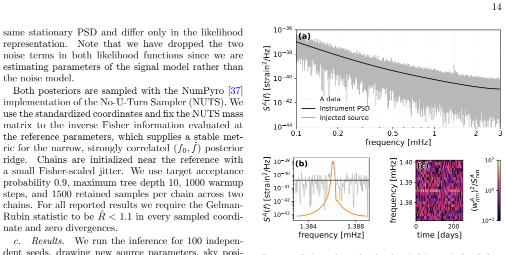
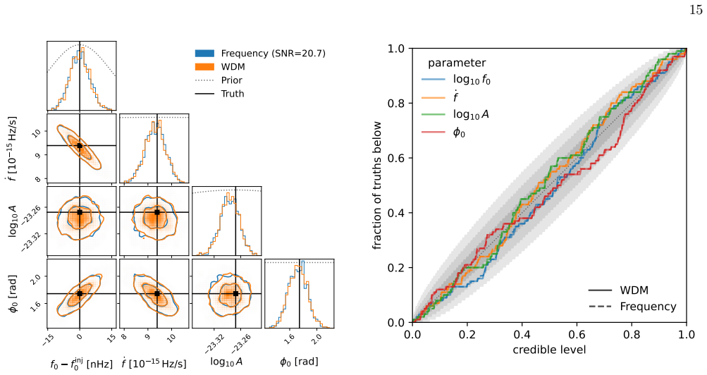
The authors show that a carefully specified, packed WDM transform, implemented with exact round-trip reconstruction, yields a WDM-domain likelihood that is numerically equivalent to the ordinary frequency-domain Whittle likelihood for resolved LISA galactic binaries when both analyses share the same stationary noise model. Across 100 independent injections the median Jensen–Shannon divergence between one-dimensional marginals is about 5e-6 bits, confirming that the two representations agree to sampling precision in that controlled setting.
What carries the argument
The packed Wilson–Daubechies–Meyer transform: an orthonormal wavelet-packet map that sends N real samples to an (Nt, Nf+1) coefficient grid (DC, interior, and Nyquist channels), with Meyer-windowed atoms, Wilson phase factors, and exact forward/inverse formulae that make the Gram matrix G†G equal the identity, enabling a diagonal WDM Whittle likelihood under local stationarity.
Load-bearing premise
The claim that noise can be treated as locally stationary so that the WDM covariance is diagonal and off-diagonal pixel correlations can be dropped; if the spectrum changes faster than the tiling scales, that diagonal likelihood fails.
What would settle it
Re-run the same LISA galactic-binary inference with a deliberately non-stationary, time-varying PSD and check whether the WDM and frequency-domain posteriors still agree to the same Jensen–Shannon tolerance; any large systematic offset would falsify the claimed numerical equivalence outside the stationary regime.
Editorial analysis
A structured set of objections, weighed in public.
Referee Report
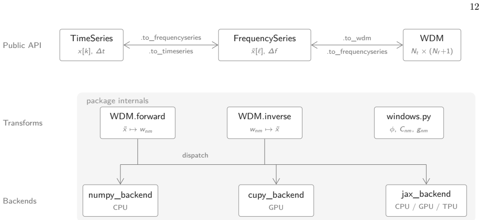
Summary. The manuscript supplies a self-contained derivation and open-source NumPy/JAX implementation of the discrete Wilson–Daubechies–Meyer (WDM) wavelet-packet transform for gravitational-wave data analysis. It fixes the packed (Nt, Nf+1) coefficient layout, the three-case Wilson basis (DC, interior, Nyquist), Meyer-window conventions, and forward/inverse formulae; proves orthonormality and the stationary diagonal-covariance approximation in the appendices; and validates floating-point-exact round-trip reconstruction. As a controlled end-to-end check, Sec. IV A shows that a WDM-domain Whittle likelihood reproduces frequency-domain posteriors for resolved LISA galactic binaries under a shared stationary noise model (median JSD ~5e-6 bits over 100 seeds).
Significance. The contribution is primarily infrastructural and pedagogical rather than a new transform or a new science result. Its value lies in making an already-used representation fully explicit, reproducible, and differentiable for modern Python/JAX inference pipelines, with GPU-accelerated million-point transforms and machine-precision round-trips. The LISA comparison is a clean numerical equivalence test under the regime where the diagonal approximation is expected to hold. The package, Zenodo archive, and pinned code links are genuine strengths that lower the barrier to adoption and to future work on non-stationary noise, gaps, and tiling optimisation that the paper itself defers.
major comments (2)
- The abstract and introduction advertise utility for non-stationary noise, stochastic backgrounds, and data gaps, yet the only end-to-end inference demonstration (Sec. IV A) uses a shared time-averaged stationary PSD in both domains. That choice correctly isolates the basis change and makes the tiny JSD expected, but it does not exercise the local-stationarity regime of Eq. (38)/App. C that is the principal statistical motivation for WDM. The paper already acknowledges this in Sec. V; the abstract and conclusions should be tightened so that the demonstrated claim (stationary numerical equivalence) is not oversold relative to the deferred non-stationary applications.
- Sec. III A–B and App. C derive the WDM Whittle likelihood and inner product after dropping DC/Nyquist channels and invoking the diagonal approximation (Eq. 38). The matrix formalism of Sec. II D correctly notes that Σw is rank-deficient when edge channels are retained. The manuscript should state more explicitly, near Eqs. (40)–(42), the quantitative conditions under which the interior-only diagonal form remains adequate for inference (e.g., spectral content near DC/Nyquist, or a bound on residual off-diagonal power after whitening), so that users know when the simple pixel-wise likelihood is safe.
minor comments (5)
- Notation for the Meyer taper parameter switches between A (main text) and a (API/package); a single convention would reduce friction for implementers.
- Fig. 2 caption and surrounding text are dense; a short sentence stating that panel (a) lives in the packed Nt(Nf+1) space while panel (b) lives in the N-dimensional signal space would help first-time readers.
- The evenness requirement on Nt and Nf is stated but not motivated beyond “left to future work”; a one-sentence remark on why the current phase/FFT construction needs it would be useful.
- A few typographical inconsistencies remain (e.g., “T erminology”, “F orward”, “ST A TISTICS”, stray /github markers in the source).
- Related WDM implementations (Digman/Cornish, Moore, Farr, cWB) are cited; a short comparison table of layout conventions and window defaults would help practitioners choose among them.
Circularity Check
No circularity: orthonormality, transforms, and diagonal covariance are derived from the basis definitions; the FD–WDM posterior match is an independent numerical check under shared stationary assumptions.
full rationale
The paper’s load-bearing mathematical claims are self-contained derivations rather than tautologies. Appendix A proves the two orthonormality relations (Eq. 16) directly from the three-case Wilson basis (Eq. 11) and the d=1 Meyer window (Eq. 12), using only the partition-of-unity property of the cosine taper and geometric-series identities; the target result is not assumed. Appendix B derives the packed forward coefficients (Eqs. 18–23) and inverse (Eq. 26) by substituting the same basis into the analysis formula and applying reality/symmetry of the DFT, again without circular substitution. Appendix C obtains the diagonal WDM covariance (Eq. 38) as a first-order approximation under wide-sense stationarity by pulling a slowly varying PSD out of the integral against the localized atoms; the approximation is stated with its failure mode (rapid PSD variation relative to ΔT, ΔF) and is not redefined as exact. The Section IV A LISA galactic-binary comparison evaluates two likelihoods (frequency-domain Whittle vs. WDM Whittle) on identical simulated data, source model, priors, and stationary PSD; the reported median JSD ~5e-6 bits is an empirical numerical equivalence check, not a quantity forced by fitting or by construction. Prior WDM literature is cited as historical background and algorithmic precedent; the present work does not import a uniqueness theorem or ansatz from overlapping authors to forbid alternatives, nor does it rename a known empirical pattern as a new prediction. Round-trip reconstruction to floating-point precision is an independent software validation of the packed layout. Consequently there are no self-definitional loops, fitted-input-as-prediction steps, or load-bearing self-citation chains.
Axiom & Free-Parameter Ledger
free parameters (3)
- Nt (number of time bins) =
example Nt=32 (LISA demo); benchmarks use Nt=1024
- A (Meyer taper width) =
default 1/3
- d (Meyer order) =
1 (fixed in current package)
axioms (4)
- standard math Discrete Fourier transform conventions and reality condition for real time series (numpy-style, zero-centered frequencies).
- domain assumption Wilson basis pairing of positive/negative frequency atoms with phase C_nm yields a real orthogonal packet basis when combined with a Meyer window.
- domain assumption Wide-sense stationary (or locally stationary) Gaussian noise with slowly varying PSD relative to the WDM pixel support, so the covariance is approximately diagonal in the WDM domain.
- ad hoc to paper Nt and Nf are even positive integers with N = Nt Nf.
read the original abstract
The Wilson-Daubechies-Meyer (WDM) time-frequency transform has been widely used in gravitational-wave astronomy, yet a self-contained, mathematically explicit reference for practitioners remains lacking. This is especially true for those wishing to adopt the transform in modern Python and JAX inference workflows. We present wdm_transform, an open-source Python package implementing the WDM wavelet-packet time-frequency transform, and document its mathematical foundations, statistical properties, and practical implementation for gravitational-wave data analysis. The package supplies NumPy and JAX backends, both transforms (forward and inverse) validated to floating-point precision, with the JAX backend enabling GPU-accelerated transforms of million-point data streams in tens of milliseconds. As a worked example, we verify that the WDM-domain likelihood reproduces frequency-domain posteriors for a resolved LISA galactic binary under a shared stationary noise model, confirming numerical equivalence of the two representations in that controlled setting. This work paves the way for systematic optimisation of WDM tilings, a particularly promising direction for the non-stationary noise, stochastic backgrounds, and data gaps anticipated in future detectors, and for direct comparisons with alternative time-frequency representations needed to meet the challenges of future gravitational-wave data analysis.
Figures



Forward citations
Cited by 1 Pith paper
-
Modeling non-stationary noise: applications in gravitational wave astronomy
A positive dynamic spectrum S(f,t) generalizes the stationary power spectrum by defining Gramian closed-form noise covariances in Fourier and Wilson-Daubechies wavelet bases for gravitational wave data.
Reference graph
Works this paper leans on
-
[1]
Wil- son
coefficient layout explicitly, spell out the DC and Nyquist channel treatment, and set the normalization, phase, and indexing conventions used by the implemen- tation. These choices are then validated through ex- act round-trip reconstruction tests – applying the for- ward transform followed by its inverse – and empiri- cal checks of coefficient decorrela...
-
[2]
(10) with the interior-channel basis element from Eq
Interior channels(0< m < N f) Starting from Eq. (10) with the interior-channel basis element from Eq. (11), the forward transform can be 3 Our definitions of the Wilson basis functions (11) carefully in- clude them= 0 andm=N f in order for orthogonality to hold. evaluated in the Fourier domain using wnm = N/2−1X l=−N/2 ˜x[l] ˜g∗ nm[l],(17) For a real-valu...
-
[3]
DC channel(m= 0) The DC edge channel has a doubled time-shift ex- ponent and noC nm factor in the basis definition (11). 7 Following the same Fourier-domain evaluation yields wn0 = √ 2ℜ Nt/2−1X l=1 ˜x[l]e4πiln/Nt ˜φ[l] + 1√ 2 ˜x[0] ˜φ[0]./github (21) Note the factor of 4πin the exponent (versus 2πfor interior channels): the DC basis element oscill...
-
[4]
Towards LISA catalogs
Nyquist channel(m=N f) The Nyquist edge channel is handled analogously to the DC channel but centered at the Nyquist frequency fmax. Its structure mirrors the DC case with appropri- ate frequency shifts. In practice, the Nyquist channel is computed using the same windowed-FFT machinery as the interior channels, with the frequency shift set to mNt/2 =N/2. ...
2023
-
[5]
Now we have to consider three cases
The second (quasi)normality condition We want to evaluate X l ˜gnm[l]˜g∗ pq[l] (A10) we immediately note that, since the window support in frequency isN t/2 we are forced to haveq=m. Now we have to consider three cases. Casem= 0, for which we have X l ˜gn0[l]˜g∗ p0[l] = 1 2 N/2−1X l=−N/2 e−4πil(n−p)/Nt ˜φ2[l] = 1 2 Nt/2−1X l=−Nt/2 e−4πil(n−p)/Nt ˜φ2[l] = ...
-
[6]
(A2) is correctly normalized
Normalization of the Meyer window We verify that the Meyer window defined in Eq. (A2) is correctly normalized. We compute N/2−1X l=−N/2 ˜φ2[l] = 2 A Nt 2 −1X l=0 2 Nt − 2 Nt + 2 (A+B) Nt 2 −1X l=A Nt 2 2 Nt cos2 " π 2 2l Nt −A B # = 2A− 2 Nt + 4 Nt B Nt 2 −1X k=0 cos2 π 2 2k BNt = = 2A− 2 Nt + 4 Nt B Nt 2 −1X k=0 1 2 + 4 Nt B Nt 2 −1X k=0 1 2 cos 2πk BNt ...
-
[7]
Interior channels(0< m < N f) Inserting the interior-channel basis element from Eq. (11) and splitting the sum over positive and negative frequencies gives wnm = 1√ 2 N/2−1X l=0 ˜x[l]e2πiln/Nt C ∗ nm ˜φ l− mNt 2 +C nm ˜φ l+ mNt 2 + 1√ 2 −1X l=−N/2 ˜x[l]e2πiln/Nt C ∗ nm ˜φ l− mNt 2 +C nm ˜φ l+ mNt 2 .(B2) Using the reality condition ˜x[−l] = ˜x[l]∗ togethe...
-
[8]
DC channel(m= 0) For the DC edge channel, the basis element has a doubled time-shift exponent and noC nm factor. The same positive/negative frequency splitting yields wn0 = 1√ 2 N/2−1X l=0 ˜x[l]e4πiln/Nt ˜φ[l] +1√ 2 −1X l=−N/2 ˜x[l]e4πiln/Nt ˜φ[l] = √ 2ℜ Nt/2−1X l=1 ˜x[l]e4πiln/Nt ˜φ[l] + 1√ 2 ˜x[0] ˜φ[0],(B4) which is Eq. (21) of the main text
-
[9]
Nyquist channel(m=N f) wnm = 1√ 2 N/2−1X l=0 ˜x[l]e4πiln/Nt ˜φ l− N 2 + ˜φ l+ N 2 + 1√ 2 −1X l=−N/2 ˜x[l]e4πiln/Nt ˜φ l− N 2 + ˜φ l+ N 2 = 1√ 2 N/2−1X l=0 ˜x[l]e4πiln/Nt ˜φ l− N 2 + ˜φ l+ N 2 + 1√ 2 N/2X l=1 ˜x[−l]e−4πiln/Nt ˜φ −l− N 2 + ˜φ −l+ N 2 .(B5) Thel= 0 term in the first summation vanishes, and thel=N/2 term is treated separately: wnm = √ 2ℜ N/2−...
-
[10]
Appendix C: The WDM Covariance Matrix in the stationary case We start from the WDM transform in Eq
The inverse transform We write the inverse transform of thew nm coefficients to recover the signal ˜x[l] forl≥0 since we know that for l <0 the reality condition holds (˜x[−l] = ˜x∗[l]): ˜x[l] = Nt−1X n=0 NfX m=0 wnmgnm[l] = 1√ 2 X n X 0<m<Nf wnme−2πiln/Nt Cnm ˜φ l− mNt 2 +C ∗ nm ˜φ l+ mNt 2 + 1√ 2 X n wn0e−4πiln/Nt ˜φ[l] +1√ 2 X n wnNf e−4πiln/Nt ˜φ l− N...
-
[11]
Kr´ olak and P
A. Kr´ olak and P. Trzaskoma, Classical and Quantum Gravity13, 813 (1996)
1996
-
[12]
Virtuoso and E
A. Virtuoso and E. Milotti, Phys. Rev. D109, 102010 (2024)
2024
-
[13]
Robinet, N
F. Robinet, N. Arnaud, N. Leroy, A. Lundgren, D. Macleod, and J. McIver, SoftwareX12, 100620 (2020)
2020
-
[14]
N. J. Cornish and T. B. Littenberg, Classical and Quantum Gravity32, 135012 (2015)
2015
-
[15]
S. Chatterji, L. Blackburn, G. Martin, and E. Katsavounidis, Class. Quant. Grav.21, S1809 (2004), arXiv:gr-qc/0412119
Pith/arXiv arXiv 2004
-
[16]
E. Chassande-Mottin and A. Pai, Phys. Rev. D73, 042003 (2006), arXiv:gr-qc/0512137
Pith/arXiv arXiv 2006
-
[17]
Gair and L
J. Gair and L. Wen, Classical and Quantum Gravity22, S1359–S1371 (2005)
2005
-
[18]
J. R. Gair, I. Mandel, and L. Wen, Class. Quant. Grav.25, 184031 (2008), arXiv:0804.1084 [gr-qc]
Pith/arXiv arXiv 2008
-
[19]
L. Speri, R. Tenorio, C. Chapman-Bird, and D. Gerosa, Physical Review D113, 10.1103/dh3j-ksfl (2026)
-
[20]
D. Bandopadhyay, C. E. A. Chapman-Bird, and A. Vecchio, Global time-frequency search for stellar-mass binary black holes in LISA (2026), arXiv:2510.19047 [gr-qc]
Pith/arXiv arXiv 2026
-
[21]
Colpiet al., arXiv e-prints , arXiv:2402.07571 (2024), arXiv:2402.07571 [astro-ph.CO]
M. Colpiet al., arXiv e-prints , arXiv:2402.07571 (2024), arXiv:2402.07571 [astro-ph.CO]
Pith/arXiv arXiv 2024
-
[22]
J. Luoet al., Class. Quant. Grav.33, 035010 (2016), arXiv:1512.02076 [astro-ph.IM]
Pith/arXiv arXiv 2016
-
[23]
N. J. Cornish, T. B. Littenberg, B. B´ ecsy, K. Chatziioannou, J. A. Clark, S. Ghonge, and M. Millhouse, Phys. Rev. D 103, 044006 (2021), arXiv:2011.09494 [gr-qc]
Pith/arXiv arXiv 2021
-
[24]
Necula, S
V. Necula, S. Klimenko, and G. Mitselmakher, Journal of Physics: Conference Series363, 012032 (2012)
2012
-
[25]
M. J. Szczepa´ nczyk, F. Salemi, S. Bini, T. Mishra, G. Vedovato, V. Gayathri, I. Bartos, S. Bhaumik, M. Drago, O. Halim, C. Lazzaro, A. Miani, E. Milotti, G. A. Prodi, S. Tiwari, and S. Klimenko, Phys. Rev. D107, 062002 (2023), arXiv:2210.01754 [gr-qc]
Pith/arXiv arXiv 2023
-
[26]
M. Drago, S. Klimenko, C. Lazzaro, E. Milotti, G. Mitselmakher, V. Necula, B. O’Brian, G. A. Prodi, F. Salemi, M. Szczepanczyk, S. Tiwari, V. Tiwari, V. Gayathri, G. Vedovato, and I. Yakushin, SoftwareX14, 100678 (2021), arXiv:2006.12604 [gr-qc]. 23
Pith/arXiv arXiv 2021
-
[27]
W. G. Anderson, P. R. Brady, J. D. E. Creighton, and E. E. Flanagan, Phys. Rev. D63, 042003 (2001), arXiv:gr- qc/0008066
arXiv 2001
-
[28]
Klimenko and G
S. Klimenko and G. Mitselmakher, Class. Quant. Grav.21, S1819 (2004)
2004
-
[29]
M. C. Digman and N. J. Cornish, WDMWaveletTransforms: Fast forward and inverse WDM wavelet transforms, Astro- physics Source Code Library, record ascl:2307.037 (2023), ascl:2307.037
2023
-
[30]
M. C. Digman and N. J. Cornish, Phys. Rev. D108, 023022 (2023), arXiv:2212.04600 [gr-qc]
Pith/arXiv arXiv 2023
-
[31]
M. C. Digman and N. J. Cornish, Astrophys. J.940, 10 (2022), arXiv:2206.14813 [astro-ph.IM]
Pith/arXiv arXiv 2022
-
[32]
N. Pearson and N. J. Cornish, Phys. Rev. D113, 064033 (2026), arXiv:2509.05479 [gr-qc]
Pith/arXiv arXiv 2026
-
[33]
N. J. Cornish, Phys. Rev. D102, 124038 (2020), arXiv:2009.00043 [gr-qc]
Pith/arXiv arXiv 2020
-
[34]
N. J. Cornish, arXiv e-prints , arXiv:2511.10632 (2025), arXiv:2511.10632 [gr-qc]
Pith/arXiv arXiv 2025
-
[35]
N. J. Cornish, WDM Transform: Codes to compute the WDM wavelet transform,https://github.com/ eXtremeGravityInstitute/WDM_Transform(2020), eXtreme Gravity Institute, Montana State University. Implements fast TaylorT, TaylorF, and sparse WDM transforms for binary chirp signals in C. Accessed: May 2026
2020
-
[36]
M. C. Digman, WDMWaveletTransforms: Fast forward and inverse WDM wavelet transforms in Python,https:// github.com/XGI-MSU/WDMWaveletTransforms(2022), eXtreme Gravity Institute, Montana State University. Produced under NASA LISA Preparatory Science Grant 80NSSC19K0320. Released v0.0.1, April 2025; GPLv2+ licence. Accessed: May 2026
2022
-
[37]
C. J. Moore, WDM GW wavelets: A fast, JAX-based Python implementation of the Wilson–Daubechies–Meyer wavelet transform for gravitational wave data,https://cjm96.github.io/WDM_GW_wavelets/(2025), gitHub repository:https: //github.com/cjm96/WDM_GW_wavelets. Includes time-delay filter routines for space-based detector responses. Accessed: May 2026
2025
-
[38]
GitLab:https://gitlab.com/gwburst/public/library
cWB Team, coherent WaveBurst (cWB), version cWB-6.4.6.0,https://gwburst.gitlab.io/documentation/latest/ html/(2024), public release used for the LVK O4b analysis. GitLab:https://gitlab.com/gwburst/public/library. GPLv3 licence. Accessed: May 2026
2024
-
[39]
W. M. Farr, WDMWavelets.jl: WDM wavelets in Julia,https://github.com/farr/WDMWavelets.jl(2025), gitHub repository
2025
-
[40]
B. Krishnan, A. M. Sintes, M. A. Papa, B. F. Schutz, S. Frasca, and C. Palomba, Phys. Rev. D70, 082001 (2004), arXiv:gr-qc/0407001
Pith/arXiv arXiv 2004
-
[41]
Palomba, P
C. Palomba, P. Astone, and S. Frasca, Classical and Quantum Gravity22, S1255 (2005)
2005
-
[42]
Savalle, J
E. Savalle, J. Gair, L. Speri, and S. Babak, Phys. Rev. D106, 022003 (2022)
2022
-
[43]
Daubechies, S
I. Daubechies, S. Jaffard, and J. L. Journe, SIAM J. Math. Anal.22, 554 (1991)
1991
-
[44]
O. Burke, S. Marsat, J. R. Gair, and M. L. Katz, Phys. Rev. D111, 124053 (2025), arXiv:2502.17426 [gr-qc]
Pith/arXiv arXiv 2025
-
[45]
N. Bartoloet al., J. Cosmol. Astropart. Phys.2022, 009 (2022), arXiv:2201.08782 [astro-ph.CO]
Pith/arXiv arXiv 2022
-
[46]
Bayle, M
J.-B. Bayle, M. Le Jeune, and J. Menu, jaxgb: Fast LISA response for Galactic binaries using JAX,https://pypi.org/ project/jaxgb/(2025), version 0.2.1, BSD-3-Clause
2025
-
[47]
D. Phan, N. Pradhan, and M. Jankowiak, arXiv e-prints , arXiv:1912.11554 (2019), arXiv:1912.11554 [stat.ML]
Pith/arXiv arXiv 1912
-
[48]
S. Klimenko, S. Mohanty, M. Rakhmanov, and G. Mitselmakher, Phys. Rev. D72, 122002 (2005), arXiv:gr-qc/0508068
Pith/arXiv arXiv 2005
-
[49]
S. Klimenkoet al., Phys. Rev. D93, 042004 (2016), arXiv:1511.05999 [gr-qc]
Pith/arXiv arXiv 2016
-
[50]
Vajpeyi, G
A. Vajpeyi, G. Mentasti, Q. Baghi, O. Burke, and L. Speri, pywavelet/wdm transform: v0.05 (2026)
2026
discussion (0)
Sign in with ORCID, Apple, or X to comment. Anyone can read and Pith papers without signing in.