BPS Dendroscopy on Local mathbb{P}¹times mathbb{P}¹
Pith reviewed 2026-05-23 06:59 UTC · model grok-4.3
The pith
The scattering diagram on local F0 determines all BPS indices from attractor indices via ray intersection consistency.
A machine-rendered reading of the paper's core claim, the machinery that carries it, and where it could break.
Core claim
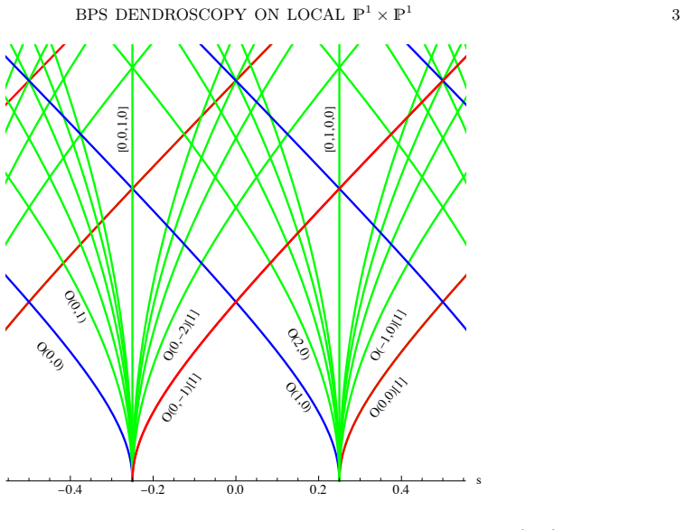
In the scattering diagram for local F0, an arrangement of rays in the space of stability conditions marks loci where BPS states of given charge and central charge phase exist; the consistency of the diagram when rays intersect determines all BPS indices in terms of the attractor indices carried by the initial rays, allowing a sketch of the proof of the Split Attractor Flow Tree Conjecture for a restricted range of the central charge phase.
What carries the argument
The scattering diagram, an arrangement of real codimension-one rays in stability condition space whose intersections enforce consistency relations on BPS indices.
If this is right
- All BPS indices on the Pi-stability slice are fixed once the attractor indices on the initial rays are known.
- The scattering diagram carries an action of a Z^4 extension of the modular group Gamma0(4).
- The construction combines the quiver description near the orbifold point with the large-volume limit to cover the physical slice.
- The extra mass parameter and ramification points on the Pi-stability slice complicate the diagram relative to the local P2 case.
Where Pith is reading between the lines
- The same ray-consistency method could be applied to other non-compact toric Calabi-Yau threefolds once their attractor indices are known.
- The presence of ramification points may indicate that the modular action on the stability slice is richer than in simpler geometries.
- If the restricted-phase sketch extends without new obstructions, it would give a systematic way to compute the full BPS spectrum from a small set of attractor data.
Load-bearing premise
The consistency arguments and conjecture sketch hold only for a restricted range of the central charge phase.
What would settle it
A mismatch between BPS indices computed directly at a point in the restricted phase range and the values fixed by enforcing consistency on the constructed scattering diagram would falsify the determination claim.
Figures


read the original abstract
BPS states in type II string compactified on a Calabi-Yau threefold can typically be decomposed as moduli-dependent bound states of absolutely stable constituents, with a hierarchical structure labelled by attractor flow trees. This decomposition is best understood from the scattering diagram, an arrangement of real codimension-one loci (or rays) in the space of stability conditions where BPS states of given electromagnetic charge and fixed phase of the central charge exist. The consistency of the diagram when rays intersect determines all BPS indices in terms of the `attractor indices' carried by the initial rays. In this work we study the scattering diagram for a non-compact toric CY threefold known as local $\mathbb{F}_0$, namely the total space of the canonical bundle over $\mathbb{P}^1\times \mathbb{P}^1$. We first construct the scattering diagram for the quiver, valid near the orbifold point, and for the large volume slice, valid when both $\mathbb{P}^1$'s have large (and nearly equal) area. We then combine the insights gained from these simple limits to construct the scattering diagram along the physical slice of $\Pi$-stability conditions, which carries an action of a $\mathbb{Z}^4$ extension of the modular group $\Gamma_0(4)$. We sketch a proof of the Split Attractor Flow Tree Conjecture in this example, albeit for a restricted range of the central charge phase. Most arguments are similar to our early study of local $\mathbb{P}^2$ [arXiv:2210.10712], but complicated by the occurence of an extra mass parameter and ramification points on the $\Pi$-stability slice.
Editorial analysis
A structured set of objections, weighed in public.
Referee Report
Summary. The paper constructs the scattering diagram for BPS states on the non-compact toric Calabi-Yau threefold local F0 (total space of the canonical bundle over P1 x P1). It first builds the diagram near the orbifold point from the quiver and at large volume for nearly equal large P1 areas, then combines these to the Pi-stability slice carrying a Z^4 extension of Gamma0(4). Diagram consistency at ray intersections is claimed to determine all BPS indices from the attractor indices on initial rays. A sketch of the Split Attractor Flow Tree Conjecture is provided, but only for a restricted range of central charge phase, with complications from an extra mass parameter and ramification points relative to the local P2 case studied in arXiv:2210.10712.
Significance. If the restricted-range sketch holds, the work extends BPS dendroscopy methods to a geometry with an extra mass parameter and modular action, giving concrete support for the conjecture via explicit ray-intersection consistency in a toric example beyond local P2. Strengths include the explicit construction combining quiver and large-volume limits on the physical slice and the handling of the Z^4 extension of Gamma0(4). This advances the understanding of attractor flow trees and BPS bound-state hierarchies in Calabi-Yau threefolds.
major comments (1)
- [Abstract] Abstract: The central claim that diagram consistency at ray intersections determines all BPS indices from attractor indices is load-bearing for the Split Attractor Flow Tree Conjecture sketch, yet the manuscript explicitly restricts the sketch to a limited range of central charge phase owing to ramification points on the Pi-stability slice and the extra mass parameter; this restriction means the determination is not shown to hold uniformly across the full physical slice.
Simulated Author's Rebuttal
We thank the referee for their careful reading and for identifying this point about the scope of the claims in the abstract. We address the major comment below.
read point-by-point responses
-
Referee: [Abstract] Abstract: The central claim that diagram consistency at ray intersections determines all BPS indices from attractor indices is load-bearing for the Split Attractor Flow Tree Conjecture sketch, yet the manuscript explicitly restricts the sketch to a limited range of central charge phase owing to ramification points on the Pi-stability slice and the extra mass parameter; this restriction means the determination is not shown to hold uniformly across the full physical slice.
Authors: We agree that the abstract presents the general principle of scattering diagram consistency while the explicit sketch and determination of indices via ray intersections is restricted to a limited range of central charge phase. The restriction arises precisely from the extra mass parameter and ramification points on the Π-stability slice, as stated in the manuscript. To remove any potential ambiguity, we will revise the abstract to tie the determination claim explicitly to the restricted range in which the Split Attractor Flow Tree Conjecture is sketched. revision: yes
Circularity Check
Minor self-citation to prior local P2 study for sketch of conjecture
specific steps
-
self citation load bearing
[Abstract]
"Most arguments are similar to our early study of local P2 [arXiv:2210.10712], but complicated by the occurence of an extra mass parameter and ramification points on the Pi-stability slice."
The sketch of the Split Attractor Flow Tree Conjecture is presented as relying on similarity to the authors' own prior paper for the core arguments, with the present work only adapting for added complications; while not fully load-bearing (new constructions are supplied), this constitutes a minor self-citation dependency for the central claim.
full rationale
The paper constructs scattering diagrams explicitly from the quiver near the orbifold point and the large-volume slice, then combines them along the Pi-stability slice using the consistency condition at ray intersections to determine BPS indices from attractor indices. This is a direct mathematical construction from stability conditions and the Split Attractor Flow Tree framework. The sole self-citation notes that most arguments are similar to the authors' prior local P2 work but does not serve as load-bearing justification; the current paper supplies the new elements (extra mass parameter, ramification points, Z^4 extension of Gamma_0(4)) and restricts the sketch to a limited central-charge phase range. No reductions by construction, fitted inputs renamed as predictions, or self-definitional steps appear.
Axiom & Free-Parameter Ledger
free parameters (1)
- extra mass parameter
axioms (1)
- domain assumption Consistency of the scattering diagram when rays intersect determines all BPS indices from attractor indices
Lean theorems connected to this paper
-
IndisputableMonolith/Foundation/RealityFromDistinction.leanreality_from_one_distinction unclear?
unclearRelation between the paper passage and the cited Recognition theorem.
The consistency of the diagram when rays intersect determines all BPS indices in terms of the attractor indices carried by the initial rays. We sketch a proof of the Split Attractor Flow Tree Conjecture in this example, albeit for a restricted range of the central charge phase.
-
IndisputableMonolith/Foundation/AlexanderDuality.leanalexander_duality_circle_linking unclear?
unclearRelation between the paper passage and the cited Recognition theorem.
C(τ,m) := η(τ)4 η(2τ)6 / η(4τ)4 √[(J4(τ)+8)/(J4(τ)+8 cos π m)] ... ramification points on the Π-stability slice
-
IndisputableMonolith/Cost/FunctionalEquation.leanwashburn_uniqueness_aczel contradicts?
contradictsCONTRADICTS: the theorem conflicts with this paper passage, or marks a claim that would need revision before publication.
extra mass parameter and ramification points ... m ∈ R
What do these tags mean?
- matches
- The paper's claim is directly supported by a theorem in the formal canon.
- supports
- The theorem supports part of the paper's argument, but the paper may add assumptions or extra steps.
- extends
- The paper goes beyond the formal theorem; the theorem is a base layer rather than the whole result.
- uses
- The paper appears to rely on the theorem as machinery.
- contradicts
- The paper's claim conflicts with a theorem or certificate in the canon.
- unclear
- Pith found a possible connection, but the passage is too broad, indirect, or ambiguous to say the theorem truly supports the claim.
Forward citations
Cited by 2 Pith papers
-
The non-perturbative topological string: from resurgence to wall-crossing of DT invariants
An isomorphism is shown between the algebra of alien derivatives acting on the topological string partition function and the Kontsevich-Soibelman Lie algebra, linking resurgence to DT wall-crossing with numerical matc...
-
The non-perturbative topological string: from resurgence to wall-crossing of DT invariants
Links resurgence of the topological string partition function to DT wall-crossing via an isomorphism of alien derivative algebras to the Kontsevich-Soibelman Lie algebra, with Borel singularities matched to specific D...
Reference graph
Works this paper leans on
-
[1]
P. Bousseau, P. Descombes, B. Le Floch, and B. Pioline, “BPS Dendroscopy on LocalP2,”Commun. Math. Phys. 405 (2024), no. 4, 108,2210.10712
-
[2]
Stability conditions on triangulated categories,
T. Bridgeland, “Stability conditions on triangulated categories,”Ann. of Math. (2)166 (2007), no. 2, 317–345
work page 2007
-
[3]
Bogomolov-Gieseker type inequality and counting invariants
Y. Toda, “Bogomolov-Gieseker type inequality and counting invariants,”1112.3411
work page internal anchor Pith review Pith/arXiv arXiv
-
[4]
S. Feyzbakhsh and R. P. Thomas, “Curve counting and S-duality,”Épijournal de Géométrie Algébrique7 (2023) 2007.03037
work page internal anchor Pith review Pith/arXiv arXiv 2023
-
[5]
S. Feyzbakhsh and R. P. Thomas, “Rankr DT theory from rank0,”2103.02915
-
[6]
Explicit formulae for rank zero DT invariants and the OSV conjecture,
S. Feyzbakhsh, “Explicit formulae for rank zero DT invariants and the OSV conjecture,”2203.10617
-
[7]
Quantum geometry, stability and modularity,
S. Alexandrov, S. Feyzbakhsh, A. Klemm, B. Pioline, and T. Schimannek, “Quantum geometry, stability and modularity,”Commun. Num. Theor. Phys.18 (2024), no. 1, 49–151,2301.08066
-
[8]
Scattering diagrams, hall algebras and stability conditions
T. Bridgeland, “Scattering diagrams, Hall algebras and stability conditions,”Alg. Geo. 4 (2017) 523–561, 1603.00416
-
[9]
Split attractor flows and the spectrum of BPS D-branes on the Quintic
F. Denef, B. R. Greene, and M. Raugas, “Split attractor flows and the spectrum of BPS D-branes on the quintic,”JHEP 05 (2001) 012, hep-th/0101135
work page internal anchor Pith review Pith/arXiv arXiv 2001
-
[10]
Split States, Entropy Enigmas, Holes and Halos
F. Denef and G. W. Moore, “Split states, entropy enigmas, holes and halos,”JHEP 1111 (2011) 129, hep-th/0702146
work page internal anchor Pith review Pith/arXiv arXiv 2011
-
[11]
Attractor flow trees, BPS indices and quivers,
S. Alexandrov and B. Pioline, “Attractor flow trees, BPS indices and quivers,”Adv. Theor. Math. Phys.23 (2019), no. 3, 627–699,1804.06928
-
[12]
The flow tree formula for Donaldson-Thomas invariants of quivers with potentials,
H. Argüz and P. Bousseau, “The flow tree formula for Donaldson-Thomas invariants of quivers with potentials,”Compositio Mathematica158 (2022), no. 12, 2206–2249,2102.11200
-
[13]
Scattering diagrams, stability conditions, and coherent sheaves onP2,
P. Bousseau, “Scattering diagrams, stability conditions, and coherent sheaves onP2,”J. Algebraic Geom.31 (2022) 593–686,1909.02985
-
[14]
Stability conditions on a non-compact Calabi-Yau threefold
T. Bridgeland, “Stability conditions on a non-compact Calabi-Yau threefold,”Commun. Math. Phys.266 (2006) 715–733,math/0509048
work page internal anchor Pith review Pith/arXiv arXiv 2006
-
[15]
The space of stability conditions on the local projective plane,
A. Bayer and E. Macri, “The space of stability conditions on the local projective plane,”Duke Math. J.160 (2011) 263–322,0912.0043
-
[16]
Tropical correspondence for smooth del Pezzo log Calabi-Yau pairs,
T. Graefnitz, “Tropical correspondence for smooth del Pezzo log Calabi-Yau pairs,”2005.14018
-
[17]
All Loop Topological String Amplitudes From Chern-Simons Theory
M. Aganagic, M. Marino, and C. Vafa, “All loop topological string amplitudes from Chern-Simons theory,” Commun. Math. Phys.247 (2004) 467–512,hep-th/0206164
work page internal anchor Pith review Pith/arXiv arXiv 2004
-
[18]
Vafa–Witten Invariants from Exceptional Collections,
G. Beaujard, J. Manschot, and B. Pioline, “Vafa–Witten Invariants from Exceptional Collections,” Commun. Math. Phys.385 (2021), no. 1, 101–226,2004.14466
-
[19]
Attractor invariants, brane tilings and crystals,
S. Mozgovoy and B. Pioline, “Attractor invariants, brane tilings and crystals,” to appear inAnn. Inst. Fourier (2025), 2012.14358
-
[20]
Instanton Particles and Monopole Strings in 5D SU(2) Supersymmetric Yang-Mills Theory,
P. Longhi, “Instanton Particles and Monopole Strings in 5D SU(2) Supersymmetric Yang-Mills Theory,” Phys. Rev. Lett.126 (2021), no. 21, 211601,2101.01681
-
[21]
Quiver Symmetries and Wall-Crossing Invariance,
F. Del Monte and P. Longhi, “Quiver Symmetries and Wall-Crossing Invariance,”Commun. Math. Phys. 398 (2023), no. 1, 89–132,2107.14255
-
[22]
The threefold way to quantum periods: WKB, TBA equations and q-Painlevé,
F. Del Monte and P. Longhi, “The threefold way to quantum periods: WKB, TBA equations and q-Painlevé,”SciPost Phys. 15 (2023), no. 3, 112,2207.07135
- [23]
-
[24]
Exponential Networks and Representations of Quivers
R. Eager, S. A. Selmani, and J. Walcher, “Exponential Networks and Representations of Quivers,”JHEP 08 (2017) 063, 1611.06177
work page internal anchor Pith review Pith/arXiv arXiv 2017
-
[25]
Exponential BPS graphs and D-brane counting on toric Calabi-Yau threefolds: Part II
S. Banerjee, P. Longhi, and M. Romo, “Exponential BPS graphs and D-brane counting on toric Calabi-Yau threefolds: Part II,”2012.09769
-
[26]
D. Gaiotto, G. W. Moore, and A. Neitzke, “Framed BPS States,”Adv. Theor. Math. Phys.17 (2013), no. 2, 241–397,1006.0146
work page internal anchor Pith review Pith/arXiv arXiv 2013
-
[27]
Wall-crossing from supersymmetric galaxies
E. Andriyash, F. Denef, D. L. Jafferis, and G. W. Moore, “Wall-crossing from supersymmetric galaxies,” JHEP 1201 (2012) 115, 1008.0030
work page internal anchor Pith review Pith/arXiv arXiv 2012
-
[28]
Quantum Calabi-Yau and Classical Crystals
A. Okounkov, N. Reshetikhin, and C. Vafa, “Quantum Calabi-Yau and classical crystals,”Prog. Math.244 (2006) 597, hep-th/0309208
work page internal anchor Pith review Pith/arXiv arXiv 2006
-
[29]
On the noncommutative Donaldson-Thomas invariants arising from brane tilings
S. Mozgovoy and M. Reineke, “On the noncommutative Donaldson-Thomas invariants arising from brane tilings,”Advances in mathematics223 (9, 2010) 1521–1544,0809.0117
work page internal anchor Pith review Pith/arXiv arXiv 2010
-
[30]
Wall crossing in local Calabi Yau manifolds
D. L. Jafferis and G. W. Moore, “Wall crossing in local Calabi Yau manifolds,”0810.4909
work page internal anchor Pith review Pith/arXiv arXiv
-
[31]
BPS invariants of semi-stable sheaves on rational surfaces
J. Manschot, “BPS invariants of semi-stable sheaves on rational surfaces,”Lett. Math. Phys.103 (2013) 895–918,1109.4861
work page internal anchor Pith review Pith/arXiv arXiv 2013
-
[32]
Fibrés stables et fibrés exceptionnels surP2,
J.-M. Drézet and J. Le Potier, “Fibrés stables et fibrés exceptionnels surP2,” inAnnales scientifiques de l’École Normale Supérieure, vol. 18, pp. 193–243. 1985. 64 BPS DENDROSCOPY ON LOCAL P1 × P1
work page 1985
-
[33]
Existence of semistable sheaves on Hirzebruch surfaces,
I. Coskun and J. Huizenga, “Existence of semistable sheaves on Hirzebruch surfaces,”Advances in Mathematics 381 (2021) 107636
work page 2021
-
[34]
Invariants of moduli spaces of stable sheaves on ruled surfaces
S. Mozgovoy, “Invariants of moduli spaces of stable sheaves on ruled surfaces,”1302.4134
work page internal anchor Pith review Pith/arXiv arXiv
-
[35]
Intersection cohomology of moduli spaces of sheaves on surfaces
J. Manschot and S. Mozgovoy, “Intersection cohomology of moduli spaces of sheaves on surfaces,” 1612.07620
work page internal anchor Pith review Pith/arXiv arXiv
-
[36]
Local Mirror Symmetry: Calculations and Interpretations
T. M. Chiang, A. Klemm, S.-T. Yau, and E. Zaslow, “Local mirror symmetry: Calculations and interpretations,”Adv. Theor. Math. Phys.3 (1999) 495–565,hep-th/9903053
work page internal anchor Pith review Pith/arXiv arXiv 1999
-
[37]
The Refined Topological Vertex
A. Iqbal, C. Kozcaz, and C. Vafa, “The Refined topological vertex,”JHEP 10 (2009) 069, hep-th/0701156
work page internal anchor Pith review Pith/arXiv arXiv 2009
-
[38]
Refined stable pair invariants for E-, M- and [p,q]-strings
M.-X. Huang, A. Klemm, and M. Poretschkin, “Refined stable pair invariants for E-, M- and[p, q]-strings,” JHEP 11 (2013) 112, 1308.0619
work page internal anchor Pith review Pith/arXiv arXiv 2013
-
[39]
Lectures on Bridgeland Stability,
E. Macrì and B. Schmidt, “Lectures on Bridgeland Stability,”1607.01262
-
[40]
Some quivers describing the derived categories of the toric del Pezzos,
M. Perling, “Some quivers describing the derived categories of the toric del Pezzos,” 2003. unpublished
work page 2003
-
[41]
D-Brane Gauge Theories from Toric Singularities and Toric Duality
B. Feng, A. Hanany, and Y.-H. He, “D-brane gauge theories from toric singularities and toric duality,”Nucl. Phys. B595 (2001) 165–200,hep-th/0003085
work page internal anchor Pith review Pith/arXiv arXiv 2001
-
[42]
Phase Structure of D-brane Gauge Theories and Toric Duality
B. Feng, A. Hanany, and Y.-H. He, “Phase structure of D-brane gauge theories and toric duality,”JHEP 08 (2001) 040, hep-th/0104259
work page internal anchor Pith review Pith/arXiv arXiv 2001
-
[43]
On 5D SCFTs and their BPS quivers. Part I: B-branes and brane tilings,
C. Closset and M. Del Zotto, “On 5D SCFTs and their BPS quivers. Part I: B-branes and brane tilings,” Adv. Theor. Math. Phys.26 (2022), no. 1, 37–142,1912.13502
-
[44]
Helices on del Pezzo surfaces and tilting Calabi–Yau algebras,
T. Bridgeland and D. Stern, “Helices on del Pezzo surfaces and tilting Calabi–Yau algebras,”Advances in Mathematics 224 (2010), no. 4, 1672–1716
work page 2010
-
[45]
Scattering diagrams of quivers with potentials and mutations,
L. Mou, “Scattering diagrams of quivers with potentials and mutations,”1910.13714
-
[46]
Bridgeland-stable moduli spaces for K-trivial surfaces,
D. Arcara, A. Bertram, and M. Lieblich, “Bridgeland-stable moduli spaces for K-trivial surfaces,”J. Eur. Math. Soc.(JEMS) 15 (2013), no. 1, 1–38
work page 2013
-
[47]
Computing the Walls Associated to Bridgeland Stability Conditions on Projective Surfaces
A. Maciocia, “Computing the walls associated to Bridgeland stability conditions on projective surfaces,” Asian Journal of Mathematics18 (2014), no. 2, 263–280,1202.4587
work page internal anchor Pith review Pith/arXiv arXiv 2014
-
[48]
Bridgeland Stability of Line Bundles on Surfaces
D. Arcara and E. Miles, “Bridgeland Stability of Line Bundles on Surfaces,”Journal of Pure and Applied Algebra 220 (2016), no. 4, 1655–1677,1401.6149
work page internal anchor Pith review Pith/arXiv arXiv 2016
-
[49]
Crossing the Wall: Branes vs. Bundles
E. Diaconescu and G. W. Moore, “Crossing the wall: Branes versus bundles,”Adv. Theor. Math. Phys.14 (2010), no. 6, 1621–1650,0706.3193
work page internal anchor Pith review Pith/arXiv arXiv 2010
-
[50]
Operadic approach to wall-crossing,
S. Mozgovoy, “Operadic approach to wall-crossing,”J. Algebra 596 (2022) 53–88,2101.07636
-
[51]
Stability structures, motivic Donaldson-Thomas invariants and cluster transformations
M. Kontsevich and Y. Soibelman, “Stability structures, motivic Donaldson-Thomas invariants and cluster transformations,”0811.2435
work page internal anchor Pith review Pith/arXiv arXiv
-
[52]
Geometric Engineering of Quantum Field Theories
S. H. Katz, A. Klemm, and C. Vafa, “Geometric engineering of quantum field theories,”Nucl. Phys. B497 (1997) 173–195,hep-th/9609239
work page internal anchor Pith review Pith/arXiv arXiv 1997
-
[53]
Matrix Model as a Mirror of Chern-Simons Theory
M. Aganagic, A. Klemm, M. Marino, and C. Vafa, “Matrix model as a mirror of Chern-Simons theory,” JHEP 02 (2004) 010, hep-th/0211098
work page internal anchor Pith review Pith/arXiv arXiv 2004
-
[54]
Integrability of the holomorphic anomaly equations
B. Haghighat, A. Klemm, and M. Rauch, “Integrability of the holomorphic anomaly equations,”JHEP 10 (2008) 097, 0809.1674
work page internal anchor Pith review Pith/arXiv arXiv 2008
-
[55]
Direct integration for general Omega backgrounds
M.-x. Huang and A. Klemm, “Direct integration for generalΩ backgrounds,”Adv. Theor. Math. Phys.16 (2012), no. 3, 805–849,1009.1126
work page internal anchor Pith review Pith/arXiv arXiv 2012
-
[56]
The Omega deformed B-model for rigid N=2 theories
M.-x. Huang, A.-K. Kashani-Poor, and A. Klemm, “TheΩ deformed B-model for rigidN = 2 theories,” Annales Henri Poincare14 (2013) 425–497,1109.5728
work page internal anchor Pith review Pith/arXiv arXiv 2013
-
[57]
Exact results for topological strings on resolved Y(p,q) singularities
A. Brini and A. Tanzini, “Exact results for topological strings on resolvedY p,q singularities,”Commun. Math. Phys. 289 (2009) 205–252,0804.2598
work page internal anchor Pith review Pith/arXiv arXiv 2009
-
[58]
TheU-plane of rank-one 4dN = 2 KK theories,
C. Closset and H. Magureanu, “TheU-plane of rank-one 4dN = 2 KK theories,”SciPost Phys. 12 (2022) 065, 2107.03509
-
[59]
H. Kim, J. Manschot, and G. Moore. to appear
-
[60]
Cutting and gluing with running couplings in N=2 QCD,
J. Aspman, E. Furrer, and J. Manschot, “Cutting and gluing with running couplings in N=2 QCD,”Phys. Rev. D 105 (2022), no. 2, 025021,2107.04600
-
[61]
Closed Sub-Monodromy Problems, Local Mirror Symmetry and Branes on Orbifolds
K. Mohri, Y. Onjo, and S.-K. Yang, “Closed submonodromy problems, local mirror symmetry and branes on orbifolds,”Rev. Math. Phys.13 (2001) 675–715,hep-th/0009072
work page internal anchor Pith review Pith/arXiv arXiv 2001
-
[62]
Monopole Condensation, And Confinement In N=2 Supersymmetric Yang-Mills Theory
N. Seiberg and E. Witten, “Electric - magnetic duality, monopole condensation, and confinement in N=2 supersymmetric Yang-Mills theory,”Nucl. Phys. B426 (1994) 19–52,hep-th/9407087. [Erratum: Nucl.Phys.B 430, 485–486 (1994)]
work page internal anchor Pith review Pith/arXiv arXiv 1994
-
[63]
Special geometry, quasi-modularity and attractor flow for BPS structures,
M. Alim, F. Beck, A. Biggs, and D. Bryan, “Special geometry, quasi-modularity and attractor flow for BPS structures,”2308.16854
-
[64]
Introduction to Seiberg-Witten theory and its stringy origin,
W. Lerche, “Introduction to Seiberg-Witten theory and its stringy origin,”Nucl. Phys. B Proc. Suppl.55 (1997) 83–117,hep-th/9611190
discussion (0)
Sign in with ORCID, Apple, or X to comment. Anyone can read and Pith papers without signing in.