LatticeVision: Image to Image Networks for Modeling Non-Stationary Spatial Data

Antony Sikorski; Daniel McKenzie; Douglas Nychka; Michael Ivanitskiy; Nathan Lenssen

arxiv: 2505.09803 · v3 · submitted 2025-05-14 · 📊 stat.ML · cs.LG

LatticeVision: Image to Image Networks for Modeling Non-Stationary Spatial Data

Antony Sikorski , Michael Ivanitskiy , Nathan Lenssen , Douglas Nychka , Daniel McKenzie This is my paper

Pith reviewed 2026-05-22 14:43 UTC · model grok-4.3

classification 📊 stat.ML cs.LG

keywords spatial autoregressive modelsimage-to-image networksnon-stationary fieldsparameter estimationneural networksspatial statisticsmachine learningSAR models

0 comments

The pith

Image-to-image networks estimate parameters for non-stationary spatial autoregressive models faster and more accurately than maximum likelihood.

A machine-rendered reading of the paper's core claim, the machinery that carries it, and where it could break.

The paper establishes that spatial autoregressive models with parameters placed on a regular grid can have both their input fields and output parameters treated as images. This allows standard image-to-image neural networks to learn the mapping from observed spatial data directly to the model parameters. A sympathetic reader cares because maximum likelihood estimation becomes computationally prohibitive for large non-stationary fields, and the network approach sidesteps that cost while handling models of greater complexity than before.

Core claim

Because the SAR parameters can be arranged on a regular grid, both the inputs consisting of spatial fields and the outputs consisting of model parameters can be viewed as images, and image-to-image networks thereby enable faster and more accurate parameter estimation for a class of non-stationary SAR models with unprecedented complexity.

What carries the argument

The image-to-image network that takes spatial field images as input and produces parameter grid images as output, learning the direct mapping that replaces maximum likelihood estimation.

If this is right

Parameter estimation becomes feasible for SAR models whose non-stationarity and scale would make maximum likelihood estimation intractable.
The same trained network can process new spatial fields in a single forward pass rather than running an iterative optimizer per field.
Model complexity can increase without a corresponding explosion in computational cost for fitting.
Spatial statistics workflows can shift from custom likelihood code to off-the-shelf image translation architectures.

Where Pith is reading between the lines

These are editorial extensions of the paper, not claims the author makes directly.

The method could be tested on other classes of spatial models whose parameters also admit a regular grid layout, such as certain Gaussian processes or random fields.
If the network outputs respect the statistical dependencies of the SAR process, downstream tasks like prediction or uncertainty quantification may inherit improved calibration without extra post-processing.
Real-time updating of spatial model parameters becomes conceivable for streaming sensor data arranged in grids.

Load-bearing premise

That SAR parameters placed on a regular grid can be treated as ordinary image outputs for standard image-to-image networks without losing the underlying statistical properties or requiring loss functions that respect the autoregressive structure.

What would settle it

A direct speed and accuracy comparison on a held-out set of large non-stationary SAR fields where the image-to-image network either matches or exceeds maximum likelihood estimation in parameter recovery error while running at least ten times faster.

Figures

Figures reproduced from arXiv: 2505.09803 by Antony Sikorski, Daniel McKenzie, Douglas Nychka, Michael Ivanitskiy, Nathan Lenssen.

**Figure 2.** Figure 2: Illustration of the effects of κ 2 , ρ, and θ. The ellipses represent contours of constant correlation, e.g. all locations with correlation 0.5 with the origin. κ 2 controls the radii of the ellipse, ρ controls the ratio of the semi-major and semi-minor radii (i.e., the ‘aspect ratio’ of the ellipse), and θ is the angle the semi-major ellipse makes with the positive x-axis. (stationarity), and depends only… view at source ↗

**Figure 3.** Figure 3: Spatial patterns and their frequencies. been chosen, we sample values from the prior distribution of the specific parameter (κ 2 , ρ, or θ) for which we are constructing a field. Each pattern (except “Constant”) requires sampling two values which dictate the maximum and minimum value across the resulting parameter field. We set uniform priors on the anisotropy parameters ρ ∼ U(1, 7) and θ ∼ U − π 2 , π … view at source ↗

**Figure 4.** Figure 4: True parameters Φ (left) are encoded into the LatticeKrig SAR model to simulate a testing sample Y , of which one replicate y (0) is displayed (top). Y is used as an input to STUN and a sliding window, local estimation strategy using CNN25, resulting in Φˆ STUN (middle), and Φˆ CNN25 (right). ence in prediction RMSE. Full results are in Appendix Tables 3, 4. Our experiments highlight three consistent tren… view at source ↗

**Figure 5.** Figure 5: Top: Standardized temperature fields drawn from the CESM1 ensemble (left), the STUN-based emulator (middle), and the CNN25-based emulator (right). Bottom: Correlations with a chosen location in the Ni˜no 3.4 region at (212◦E, 1◦N) for the same three ensembles. The STUN-based emulator better preserves spatial relationships, including the zonal correlation structure along the equator and the meridional ocean… view at source ↗

**Figure 6.** Figure 6: The first replicate in a training sample ( [PITH_FULL_IMAGE:figures/full_fig_p018_6.png] view at source ↗

read the original abstract

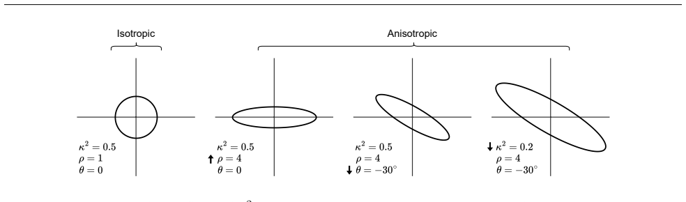
In many applications, we wish to fit a parametric statistical model to a small ensemble of spatially distributed random variables ('fields'). However, parameter inference using maximum likelihood estimation (MLE) is computationally prohibitive, especially for large, non-stationary fields. Thus, many recent works train neural networks to estimate parameters given spatial fields as input, sidestepping MLE completely. In this work we focus on a popular class of parametric, spatially autoregressive (SAR) models. We make a simple yet impactful observation; because the SAR parameters can be arranged on a regular grid, both inputs (spatial fields) and outputs (model parameters) can be viewed as images. Using this insight, we demonstrate that image-to-image (I2I) networks enable faster and more accurate parameter estimation for a class of non-stationary SAR models with unprecedented complexity.

Editorial analysis

A structured set of objections, weighed in public.

Desk editor's note, referee report, simulated authors' rebuttal, and a circularity audit. Tearing a paper down is the easy half of reading it; the pith above is the substance, this is the friction.

Desk Editor's Note private letter to a colleague

By casting SAR parameter estimation as image-to-image regression, this paper provides a practical method for fitting complex non-stationary models at scale, but it needs stronger checks that the outputs respect the model's statistical structure.

read the letter

The main thing to know is that this work reframes parameter estimation for non-stationary SAR models as an image-to-image translation task, which opens the door to handling much richer spatial variation than maximum likelihood can manage on large grids. What is new is the simple insight that both the input spatial fields and the output parameter fields can be viewed as images when the parameters are arranged on the same regular grid. This allows direct application of established I2I networks without custom architectures for the autoregressive structure. The paper shows results on models with higher complexity than previous approaches, claiming better speed and accuracy. This is a solid practical contribution for anyone dealing with spatial data where non-stationarity is key, such as in climate or ecological modeling. By avoiding the intractable MLE step, it provides a route to fitting models that capture local dependencies more flexibly. On the soft spots, the main one is around the loss function and what it actually optimizes. The stress-test concern is valid: if the network is trained with typical image losses on the parameter values, it may not penalize errors that affect the overall precision matrix or the conditional distributions in the SAR process. I would want to see whether the authors include checks that go beyond parameter error, like comparing the covariance implied by the estimated parameters to the empirical one from the data, or generating new fields and evaluating their statistical properties. Without that, the reported improvements might not fully translate to better model fits. The citation pattern looks reasonable, building on prior neural approaches to spatial parameter estimation while adding the I2I angle. This paper is for spatial statisticians and machine learning researchers focused on scalable inference for spatial processes. It would be of interest to those looking for alternatives to traditional fitting methods in high-dimensional settings. I think it deserves a serious referee. The idea is clear and the problem it tackles is important, so it should get a full review to sort out the validation questions.

Referee Report

2 major / 2 minor

Summary. The manuscript proposes LatticeVision, an image-to-image (I2I) neural network framework for parameter estimation in non-stationary spatially autoregressive (SAR) models. By arranging both the input spatial fields and the spatially varying SAR parameters on regular grids, the authors treat the problem as an image-to-image translation task, claiming that standard I2I architectures yield faster and more accurate estimates than maximum likelihood estimation (MLE) for fields of unprecedented complexity.

Significance. If the central claims are substantiated, the work would offer a computationally scalable route to inference for non-stationary spatial models that are currently intractable under MLE, with potential applications in geostatistics, environmental modeling, and spatial machine learning. The core observation that parameter grids can be viewed as images is a straightforward but useful reframing that could extend to other lattice-based spatial processes.

major comments (2)

[§3] §3 (Methods), training objective: the loss is described as a standard pixel-wise or perceptual loss on the output parameter grid. This does not include any term that penalizes mismatch between the joint distribution implied by the estimated SAR parameters and the observed data (e.g., via the precision matrix or conditional distributions), which is required to guarantee that low per-pixel parameter error translates into statistically valid SAR realizations.
[§4] §4 (Experiments), baseline comparison: the reported accuracy gains over MLE are presented without quantitative assessment of whether the network outputs reproduce the correct covariance structure or predictive distributions on held-out fields; per-parameter RMSE alone is insufficient to support the claim of 'more accurate parameter estimation' for the underlying stochastic process.

minor comments (2)

[Introduction] Notation for the non-stationary SAR model (e.g., the definition of the local autoregressive coefficients and the global precision matrix) should be introduced with an explicit equation in the introduction or early methods section for readers unfamiliar with the model class.
[Figures] Figure captions for the synthetic and real-data examples should include the exact network architecture, loss weights, and training set size to allow direct reproduction.

Simulated Author's Rebuttal

2 responses · 0 unresolved

We thank the referee for their constructive and insightful comments, which help clarify the strengths and potential improvements of our work on LatticeVision for non-stationary SAR parameter estimation. We address each major comment below, indicating planned revisions where appropriate.

read point-by-point responses

Referee: [§3] §3 (Methods), training objective: the loss is described as a standard pixel-wise or perceptual loss on the output parameter grid. This does not include any term that penalizes mismatch between the joint distribution implied by the estimated SAR parameters and the observed data (e.g., via the precision matrix or conditional distributions), which is required to guarantee that low per-pixel parameter error translates into statistically valid SAR realizations.

Authors: We appreciate this point. Our approach is fully supervised: each training field is generated from known ground-truth SAR parameters on the grid, so the network learns the inverse mapping directly. In this controlled setting, a parameter-level loss is the standard and efficient choice for estimation accuracy. That said, we agree that explicit validation of the implied joint distribution strengthens the claims of statistical validity. In the revision we will add a dedicated subsection in §3 discussing post-training checks (e.g., comparing the precision matrix or conditional distributions of generated realizations) and will include a lightweight distribution-matching regularizer as an optional extension. revision: partial
Referee: [§4] §4 (Experiments), baseline comparison: the reported accuracy gains over MLE are presented without quantitative assessment of whether the network outputs reproduce the correct covariance structure or predictive distributions on held-out fields; per-parameter RMSE alone is insufficient to support the claim of 'more accurate parameter estimation' for the underlying stochastic process.

Authors: We concur that per-parameter RMSE alone does not fully demonstrate fidelity to the underlying stochastic process. Where MLE remains tractable (smaller grids), we will augment the experimental tables with additional metrics: the Frobenius norm between estimated and true precision matrices, empirical covariance mismatch on held-out fields, and predictive log-likelihood scores. These will be reported alongside the existing RMSE results to provide a more complete picture of estimation quality. revision: yes

Circularity Check

0 steps flagged

No circularity: I2I application to SAR grids is a methodological observation, not a self-referential derivation

full rationale

The paper's core step is the observation that SAR parameters on a regular grid can be viewed as images, allowing direct use of I2I networks for parameter estimation. This is an architectural and representational choice justified by the data structure itself, not a derivation that reduces to fitted parameters or prior self-citations by construction. No equations or claims in the provided text equate outputs to inputs via self-definition, fitted-input renaming, or load-bearing self-citation chains. Empirical accuracy claims would rest on external validation against MLE or other baselines rather than internal consistency alone. The approach is self-contained against the stated goal of faster estimation for complex non-stationary SAR models.

Axiom & Free-Parameter Ledger

0 free parameters · 0 axioms · 0 invented entities

Review performed on abstract only; full paper details on network architecture, loss functions, and training data are unavailable, limiting the ability to list specific free parameters or axioms.

pith-pipeline@v0.9.0 · 5683 in / 1027 out tokens · 27578 ms · 2026-05-22T14:43:05.533878+00:00 · methodology

discussion (0)

Forward citations

Cited by 1 Pith paper

Reviewed papers in the Pith corpus that reference this work. Sorted by Pith novelty score.

A Non-stationary, Amortized, Transfer Learning Approach for Modeling Italian Air Quality
stat.AP 2026-04 unverdicted novelty 7.0

A neural network learns non-stationary anisotropic correlations from gridded CTM outputs and transfers the structure via LatticeKrig basis functions to station data for refined fine-scale NO2 predictions with uncertainty.

Reference graph

Works this paper leans on

12 extracted references · 12 canonical work pages · cited by 1 Pith paper · 1 internal anchor

[1]

Fast Gaussian process estimation for large- scale in situ inference using convolutional neural net- works

Banesh, Divya, Nishant Panda, Ayan Biswas, Luke Van Roekel, Diane Oyen, Nathan Urban, Michael Grosskopf, Jonathan Wolfe, and Earl Lawrence (2021). “Fast Gaussian process estimation for large- scale in situ inference using convolutional neural net- works”. In:2021 IEEE International Conference on Big Data (Big Data). IEEE, pp. 3731–3739. Bao, Yujia, Sriniv...

work page arXiv 2021
[2]

Diffesm: Conditional em- ulation of earth system models with diffusion mod- els

Bassetti, Seth, Brian Hutchinson, Claudia Tebaldi, and Ben Kravitz (2023). “Diffesm: Conditional em- ulation of earth system models with diffusion mod- els”. In:arXiv preprint arXiv:2304.11699. Bi, Kaifeng, Lingxi Xie, Hengheng Zhang, Xin Chen, Xiaotao Gu, and Qi Tian (2023). “Accurate medium-range global weather forecasting with 3D neural networks”. In:N...

work page arXiv 2023
[3]

Learning non-Gaussian spatial distributions via Bayesian transport maps with parametric shrink- age

Chakraborty, Anirban and Matthias Katzfuss (2025). “Learning non-Gaussian spatial distributions via Bayesian transport maps with parametric shrink- age”. In:Journal of Agricultural, Biological and En- vironmental Statistics, pp. 1–19. Chapman, William E, John S Schreck, Yingkai Sha, David John Gagne II, Dhamma Kimpara, Laure Zanna, Kirsten J Mayer, and Ju...

work page arXiv 2025
[4]

Gaussian Error Linear Units (GELUs)

Eyring, Veronika, William D Collins, Pierre Gentine, Elizabeth A Barnes, Marcelo Barreiro, Tom Beu- cler, Marc Bocquet, Christopher S Bretherton, Han- nah M Christensen, Katherine Dagon, et al. (2024). “Pushing the frontiers in climate modelling and analysis with machine learning”. In:Nature Climate Change14.9, pp. 916–928. Fuentes, Montserrat (2002). “Sp...

work page internal anchor Pith review Pith/arXiv arXiv 2024
[5]

Forecasting global weather with graph neural networks

Keisler, Ryan (2022). “Forecasting global weather with graph neural networks”. In:arXiv preprint arXiv:2202.07575. Kim, Soohyun, Jongbeom Baek, Jihye Park, Gyeongnyeon Kim, and Seungryong Kim (2022). “InstaFormer: Instance-aware image-to-image translation with transformer”. In:Proceedings of the IEEE/CVF conference on computer vision and pattern recogniti...

work page arXiv 2022
[6]

How large does a large ensemble need to be?

Springer Science & Business Media. Milinski, Sebastian, Nicola Maher, and Dirk Olon- scheck (2020). “How large does a large ensemble need to be?” In:Earth System Dynamics11.4, pp. 885–901. Nathaniel, Juan, Yongquan Qu, Tung Nguyen, Sung- duk Yu, Julius Busecke, Aditya Grover, and Pierre Gentine (2024). “Chaosbench: A multi- channel, physics-based benchmar...

work page arXiv 2020
[7]

Probablistic Emulation of a Global Cli- mate Model with Spherical DYffusion

Springer, pp. 234–241. R¨ uhling Cachay, Salva, Brian Henn, Oliver Watt- Meyer, Christopher S Bretherton, and Rose Yu (2024). “Probablistic Emulation of a Global Cli- mate Model with Spherical DYffusion”. In:Ad- vances in Neural Information Processing Systems 37, pp. 127610–127644. R¨ uhling Cachay, Salva, Bo Zhao, Hailey Joren, and Rose Yu (2023). “Dyffu...

work page arXiv 2024
[8]

The importance of internal climate variability in climate impact projections

Schwarzwald, Kevin and Nathan Lenssen (2022). “The importance of internal climate variability in climate impact projections”. In:Proceedings of the National Academy of Sciences119.42, e2208095119. Shi, Jimeng, Bowen Jin, Jiawei Han, and Giri Narasimhan (2024). “Codicast: Conditional diffusion model for weather prediction with uncertainty quantification”. ...

work page arXiv 2022
[9]

ClimateBench v1.0: A bench- mark for data-driven climate projections

Watson-Parris, Duncan, Yuhan Rao, Dirk Olivi´ e, Øyvind Seland, Peer Nowack, Gustau Camps-Valls, Philip Stier, Shahine Bouabid, Maura Dewey, Emilie Fons, et al. (2022). “ClimateBench v1.0: A bench- mark for data-driven climate projections”. In:Jour- nal of Advances in Modeling Earth Systems14.10, e2021MS002954. Watt-Meyer, Oliver, Gideon Dresdner, Jeremy ...

work page arXiv 2022
[10]

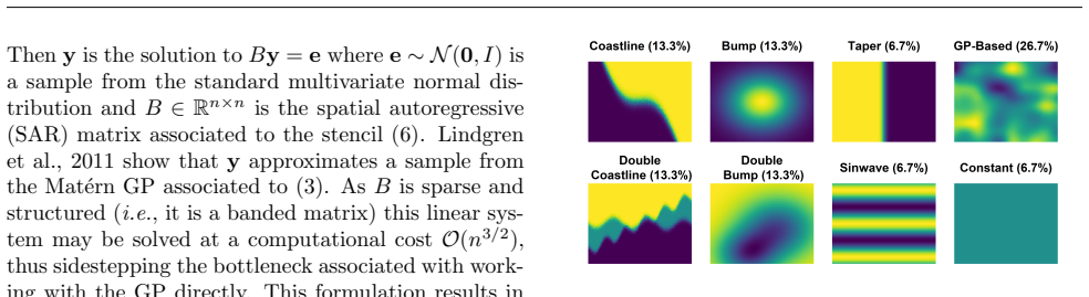
An example spatial field and its associated parameter fields can be seen in Figure

The non-stationarity in our problem does not allow for more sophisticated normalization techniques (Sikorski et al., 2024), which either become computationally intractable, require a stationary structure, or are not applicable in this setting. An example spatial field and its associated parameter fields can be seen in Figure

work page 2024
[11]

Net Reps Param Metrics RMSE↓MAE↓SSIM (↑to

PSNR↑NRMSE↓ ViT None κ2 0.398 0.279 0.252 10.9 0.040 ρ0.711 0.525 0.277 6.41 0.118 θ0.249 0.124 0.251 13.6 0.083 Sinusoidal κ2 0.393 0.274 0.275 10.8 0.040 ρ0.913 0.723 0.294 3.61 0.152 θ0.280 0.143 0.253 12.4 0.094 Learned κ2 0.371 0.2430.29112.1 0.037 ρ0.920 0.715 0.288 3.30 0.153 θ0.351 0.193 0.235 9.83 0.117 Rotary κ2 0.374 0.2500.31011.9 0.038 ρ0.625...

work page arXiv 1900
[12]

We pass the standardized ensembles of temperature sensitivity anomalies into each of our estimation networks: STUN, UNet, ViT, CNN25, CNN17, and CNN9

PSNR↑NRMSE↓ CNN9 1 κ2 1.01 0.637 0.069 4.64 0.101 ρ1.39 1.09 0.02 -0.980 0.231 θ0.535 0.295 0.072 5.27 0.179 5 κ2 0.983 0.547 0.129 6.97 0.099 ρ1.03 0.760 0.052 2.02 0.172 θ0.346 0.149 0.217 10.5 0.116 15 κ2 0.949 0.512 0.160 7.81 0.096 ρ0.962 0.689 0.070 2.90 0.160 θ0.330 0.135 0.300 11.3 0.110 30 κ2 0.963 0.508 0.172 8.09 0.097 ρ0.937 0.660 0.085 3.28 0...

work page 2019

[1] [1]

Fast Gaussian process estimation for large- scale in situ inference using convolutional neural net- works

Banesh, Divya, Nishant Panda, Ayan Biswas, Luke Van Roekel, Diane Oyen, Nathan Urban, Michael Grosskopf, Jonathan Wolfe, and Earl Lawrence (2021). “Fast Gaussian process estimation for large- scale in situ inference using convolutional neural net- works”. In:2021 IEEE International Conference on Big Data (Big Data). IEEE, pp. 3731–3739. Bao, Yujia, Sriniv...

work page arXiv 2021

[2] [2]

Diffesm: Conditional em- ulation of earth system models with diffusion mod- els

Bassetti, Seth, Brian Hutchinson, Claudia Tebaldi, and Ben Kravitz (2023). “Diffesm: Conditional em- ulation of earth system models with diffusion mod- els”. In:arXiv preprint arXiv:2304.11699. Bi, Kaifeng, Lingxi Xie, Hengheng Zhang, Xin Chen, Xiaotao Gu, and Qi Tian (2023). “Accurate medium-range global weather forecasting with 3D neural networks”. In:N...

work page arXiv 2023

[3] [3]

Learning non-Gaussian spatial distributions via Bayesian transport maps with parametric shrink- age

Chakraborty, Anirban and Matthias Katzfuss (2025). “Learning non-Gaussian spatial distributions via Bayesian transport maps with parametric shrink- age”. In:Journal of Agricultural, Biological and En- vironmental Statistics, pp. 1–19. Chapman, William E, John S Schreck, Yingkai Sha, David John Gagne II, Dhamma Kimpara, Laure Zanna, Kirsten J Mayer, and Ju...

work page arXiv 2025

[4] [4]

Gaussian Error Linear Units (GELUs)

Eyring, Veronika, William D Collins, Pierre Gentine, Elizabeth A Barnes, Marcelo Barreiro, Tom Beu- cler, Marc Bocquet, Christopher S Bretherton, Han- nah M Christensen, Katherine Dagon, et al. (2024). “Pushing the frontiers in climate modelling and analysis with machine learning”. In:Nature Climate Change14.9, pp. 916–928. Fuentes, Montserrat (2002). “Sp...

work page internal anchor Pith review Pith/arXiv arXiv 2024

[5] [5]

Forecasting global weather with graph neural networks

Keisler, Ryan (2022). “Forecasting global weather with graph neural networks”. In:arXiv preprint arXiv:2202.07575. Kim, Soohyun, Jongbeom Baek, Jihye Park, Gyeongnyeon Kim, and Seungryong Kim (2022). “InstaFormer: Instance-aware image-to-image translation with transformer”. In:Proceedings of the IEEE/CVF conference on computer vision and pattern recogniti...

work page arXiv 2022

[6] [6]

How large does a large ensemble need to be?

Springer Science & Business Media. Milinski, Sebastian, Nicola Maher, and Dirk Olon- scheck (2020). “How large does a large ensemble need to be?” In:Earth System Dynamics11.4, pp. 885–901. Nathaniel, Juan, Yongquan Qu, Tung Nguyen, Sung- duk Yu, Julius Busecke, Aditya Grover, and Pierre Gentine (2024). “Chaosbench: A multi- channel, physics-based benchmar...

work page arXiv 2020

[7] [7]

Probablistic Emulation of a Global Cli- mate Model with Spherical DYffusion

Springer, pp. 234–241. R¨ uhling Cachay, Salva, Brian Henn, Oliver Watt- Meyer, Christopher S Bretherton, and Rose Yu (2024). “Probablistic Emulation of a Global Cli- mate Model with Spherical DYffusion”. In:Ad- vances in Neural Information Processing Systems 37, pp. 127610–127644. R¨ uhling Cachay, Salva, Bo Zhao, Hailey Joren, and Rose Yu (2023). “Dyffu...

work page arXiv 2024

[8] [8]

The importance of internal climate variability in climate impact projections

Schwarzwald, Kevin and Nathan Lenssen (2022). “The importance of internal climate variability in climate impact projections”. In:Proceedings of the National Academy of Sciences119.42, e2208095119. Shi, Jimeng, Bowen Jin, Jiawei Han, and Giri Narasimhan (2024). “Codicast: Conditional diffusion model for weather prediction with uncertainty quantification”. ...

work page arXiv 2022

[9] [9]

ClimateBench v1.0: A bench- mark for data-driven climate projections

Watson-Parris, Duncan, Yuhan Rao, Dirk Olivi´ e, Øyvind Seland, Peer Nowack, Gustau Camps-Valls, Philip Stier, Shahine Bouabid, Maura Dewey, Emilie Fons, et al. (2022). “ClimateBench v1.0: A bench- mark for data-driven climate projections”. In:Jour- nal of Advances in Modeling Earth Systems14.10, e2021MS002954. Watt-Meyer, Oliver, Gideon Dresdner, Jeremy ...

work page arXiv 2022

[10] [10]

An example spatial field and its associated parameter fields can be seen in Figure

The non-stationarity in our problem does not allow for more sophisticated normalization techniques (Sikorski et al., 2024), which either become computationally intractable, require a stationary structure, or are not applicable in this setting. An example spatial field and its associated parameter fields can be seen in Figure

work page 2024

[11] [11]

Net Reps Param Metrics RMSE↓MAE↓SSIM (↑to

PSNR↑NRMSE↓ ViT None κ2 0.398 0.279 0.252 10.9 0.040 ρ0.711 0.525 0.277 6.41 0.118 θ0.249 0.124 0.251 13.6 0.083 Sinusoidal κ2 0.393 0.274 0.275 10.8 0.040 ρ0.913 0.723 0.294 3.61 0.152 θ0.280 0.143 0.253 12.4 0.094 Learned κ2 0.371 0.2430.29112.1 0.037 ρ0.920 0.715 0.288 3.30 0.153 θ0.351 0.193 0.235 9.83 0.117 Rotary κ2 0.374 0.2500.31011.9 0.038 ρ0.625...

work page arXiv 1900

[12] [12]

We pass the standardized ensembles of temperature sensitivity anomalies into each of our estimation networks: STUN, UNet, ViT, CNN25, CNN17, and CNN9

PSNR↑NRMSE↓ CNN9 1 κ2 1.01 0.637 0.069 4.64 0.101 ρ1.39 1.09 0.02 -0.980 0.231 θ0.535 0.295 0.072 5.27 0.179 5 κ2 0.983 0.547 0.129 6.97 0.099 ρ1.03 0.760 0.052 2.02 0.172 θ0.346 0.149 0.217 10.5 0.116 15 κ2 0.949 0.512 0.160 7.81 0.096 ρ0.962 0.689 0.070 2.90 0.160 θ0.330 0.135 0.300 11.3 0.110 30 κ2 0.963 0.508 0.172 8.09 0.097 ρ0.937 0.660 0.085 3.28 0...

work page 2019