Mapping atmospheric features of the planetary-mass brown dwarf SIMP 0136 with JWST NIRISS
Pith reviewed 2026-05-18 19:08 UTC · model grok-4.3
The pith
JWST spectroscopy shows the brown dwarf SIMP 0136 has three atmospheric layers whose cloud and water changes produce distinct variability patterns.
A machine-rendered reading of the paper's core claim, the machinery that carries it, and where it could break.
Core claim
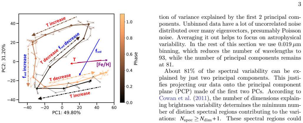
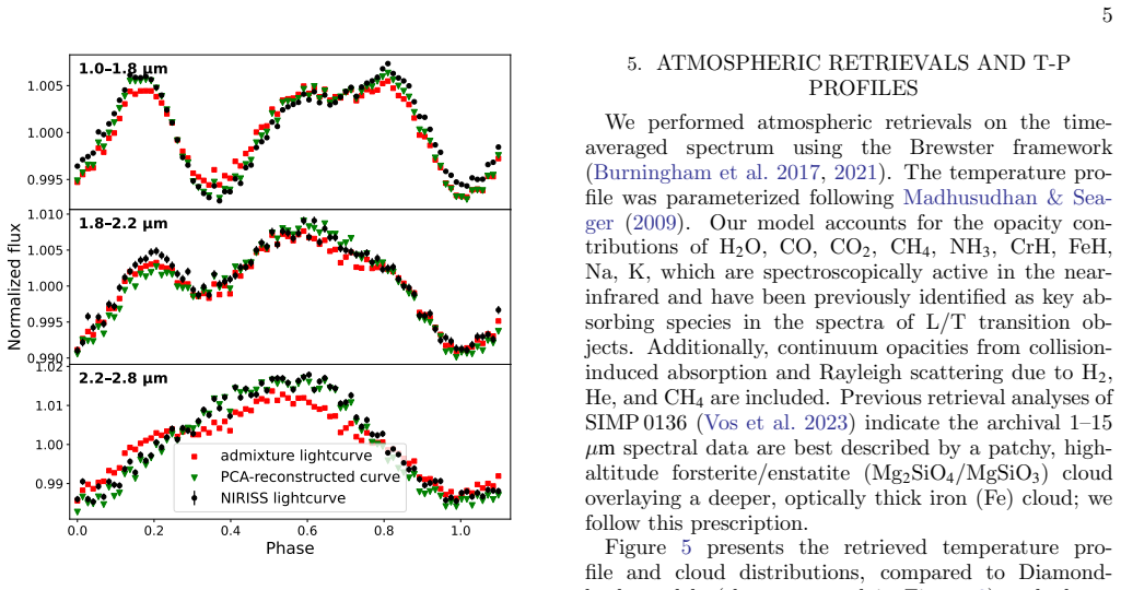
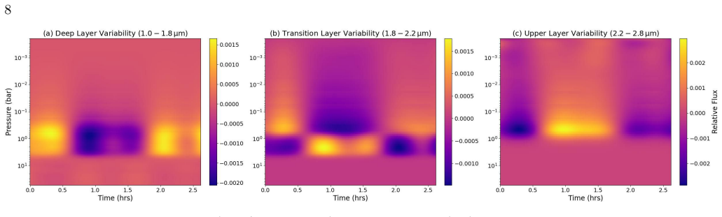
Principal component analysis reveals that 81% of spectral variations can be described by two components, implying that variability within a single rotational phase is induced by at least three distinct spectral regions. Projecting Sonora Diamondback models onto the principal component plane shows that the overall variability is highly correlated with changes in temperature, cloud coverage, and possibly effective metallicity. A combined multidimensional analysis of spectro-photometric variability links the three spectral regions to three atmospheric layers. Forsterite cloud and water abundance at each level form unique harmonics of atmospheric variability observed in different spectral bands.
What carries the argument
Principal component analysis of the time-series spectra, followed by linear combination of Sonora Diamondback models and extraction of multi-wavelength spherical harmonics brightness maps.
If this is right
- The time-averaged spectrum requires a linear combination of at least three atmospheric regions.
- Variability in different spectral bands arises from distinct vertical layers.
- Brightness maps extracted from the light curve reveal north-south asymmetry.
- Atmospheric retrievals favor an optically thick iron cloud deck beneath a patchy forsterite layer.
- Doppler shifts in the spectra can be used to help constrain the brightness maps.
Where Pith is reading between the lines
- The same layered-variability approach could be applied to time-series spectra of directly imaged giant planets.
- Higher spectral resolution or multi-rotation coverage would reduce the mapping degeneracy noted in the paper.
- If the three-layer picture holds, similar objects should show band-dependent phase curves whose amplitudes and shapes follow the same harmonic pattern.
Load-bearing premise
The two principal components extracted from the spectral time series directly trace three physically distinct atmospheric layers rather than data artifacts or unmodeled effects.
What would settle it
A single Sonora Diamondback model that reproduces the time-averaged spectrum to within the noise level without needing a linear combination of multiple regions, or principal components that show no correlation with the temperature and cloud parameters in the model grid.
Figures






read the original abstract
In this paper, we analyze James Webb Space Telescope Near Infrared Imager and Slitless Spectrograph time-series spectroscopy data to characterize the atmosphere of the planetary-mass brown dwarf SIMP J01365662+093347. Principal component analysis reveals that 81\% of spectral variations can be described by two components, implying that variability within a single rotational phase is induced by at least three distinct spectral regions. By comparing our data to a grid of Sonora Diamondback atmospheric models, we confirm that the time-averaged spectrum cannot be explained by a single model but require a linear combination of at least three regions. Projecting these models onto the principal component plane shows that the overall variability is highly correlated with changes in temperature, cloud coverage, and possibly effective metallicity. We also extract brightness maps from the lightcurve and establish North-South asymmetry in the atmosphere. A combined multidimensional analysis of spectro-photometric variability links the three spectral regions to three atmospheric layers. Forsterite cloud and water abundance at each level form unique harmonics of atmospheric variability observed in different spectral bands. Atmospheric retrievals on the time-averaged spectrum are consistent with an optically thick iron cloud deck beneath a patchy forsterite cloud layer and with the overall adiabatic curve. We also demonstrate two new analysis methods: a regionally-resolved spectra retrieval that relies on multi-wavelength spherical harmonics maps, and a method to constrain brightness maps using Doppler information present in the spectra. Future observations of variable brown dwarfs of higher spectral resolution or spanning multiple rotations should help break mapping degeneracy.
Editorial analysis
A structured set of objections, weighed in public.
Referee Report
Summary. The paper analyzes JWST NIRISS time-series spectroscopy of the planetary-mass brown dwarf SIMP J01365662+093347. Principal component analysis shows that two components capture 81% of the spectral variations, implying variability within one rotational phase arises from at least three distinct spectral regions. Comparison to the Sonora Diamondback grid indicates the time-averaged spectrum requires a linear combination of at least three regions; projection of models onto the PC plane correlates variability with temperature, cloud coverage, and metallicity. Brightness maps extracted from the light curve show North-South asymmetry. A multidimensional analysis links the three regions to three atmospheric layers where forsterite cloud and water abundances produce band-specific variability harmonics. Retrievals on the averaged spectrum support an optically thick iron cloud deck beneath patchy forsterite, consistent with an adiabatic profile. New methods are demonstrated for regionally-resolved retrievals via multi-wavelength spherical harmonics maps and for constraining brightness maps with Doppler information in the spectra.
Significance. If the vertical-layer interpretation holds, the work offers a new multidimensional framework for interpreting spectro-photometric variability in brown dwarfs and directly connects observed harmonics to specific cloud species and abundances at different levels. The use of an external model grid (Sonora Diamondback) for projection and the demonstration of two new analysis techniques (regionally-resolved retrievals and Doppler-constrained mapping) are clear strengths that could be generalized to other JWST variable-object datasets.
major comments (1)
- [Abstract and multidimensional analysis] Abstract and multidimensional analysis section: the central claim that the two principal components (plus mean) define three spectral regions that physically correspond to vertically distinct atmospheric layers rests on associating spectral features with layers, but no contribution-function calculations or pressure-level assignments are reported for the variable components. This is load-bearing for the assertion that forsterite cloud and water abundances at each level form unique harmonics; without explicit depth validation the regions could instead reflect horizontal heterogeneity, correlated parameters, or model assumptions.
minor comments (2)
- [Methods] Methods section: additional details are needed on error-bar treatment, any data exclusion criteria, and full validation steps for the PCA decomposition to allow independent reproduction of the 81% variance result.
- [Results] Figure captions and text: clarify how the North-South asymmetry in the brightness maps is quantified and whether it is statistically significant after accounting for mapping degeneracies.
Simulated Author's Rebuttal
We thank the referee for their constructive and detailed review of our manuscript on the atmospheric mapping of SIMP 0136. We address the single major comment below and will incorporate revisions to strengthen the vertical-layer interpretation.
read point-by-point responses
-
Referee: Abstract and multidimensional analysis section: the central claim that the two principal components (plus mean) define three spectral regions that physically correspond to vertically distinct atmospheric layers rests on associating spectral features with layers, but no contribution-function calculations or pressure-level assignments are reported for the variable components. This is load-bearing for the assertion that forsterite cloud and water abundances at each level form unique harmonics; without explicit depth validation the regions could instead reflect horizontal heterogeneity, correlated parameters, or model assumptions.
Authors: We appreciate the referee identifying this as a load-bearing aspect of the multidimensional analysis. The linkage of the three spectral regions to vertically distinct layers is currently supported by (i) the projection of the Sonora Diamondback grid onto the PC plane, where model variations in temperature, forsterite cloud coverage, and metallicity align with the observed PCs, and (ii) the retrieval results on the time-averaged spectrum that recover an optically thick iron cloud deck beneath patchy forsterite consistent with an adiabatic profile. These elements provide indirect depth information because the models have known pressure-dependent opacities. However, we agree that explicit contribution-function calculations and pressure-level assignments for the variable components were not reported and would help rule out purely horizontal heterogeneity or parameter correlations. In the revised manuscript we will add a dedicated subsection that computes contribution functions for the dominant spectral features of each PC using the Sonora models, assigns approximate pressure levels, and discusses how these support the unique harmonic signatures of forsterite and water at different depths. This addition will also clarify the distinction from horizontal effects already hinted at by the North-South asymmetry in the brightness maps. revision: yes
Circularity Check
No significant circularity in the derivation chain
full rationale
The paper applies PCA directly to JWST time-series spectroscopy data, finding that two components explain 81% of variance and thereby inferring at least three spectral regions via the standard linear decomposition (mean plus two PCs). It then compares the time-averaged spectrum and projected variability to an independent external grid of Sonora Diamondback atmospheric models to correlate changes with temperature, cloud coverage, and metallicity. Atmospheric retrievals on the averaged spectrum and extraction of brightness maps provide additional independent constraints. The interpretive step linking the three spectral regions to three atmospheric layers via multidimensional analysis does not reduce to a self-definition, fitted input renamed as prediction, or load-bearing self-citation; it rests on associating observed spectral features with physical parameters from the model grid rather than assuming the conclusion in the inputs. No ansatzes or uniqueness theorems from prior self-work are invoked as forcing the result. The chain is self-contained against external data and models.
Axiom & Free-Parameter Ledger
free parameters (2)
- Number of distinct spectral regions =
3
- Model parameters for temperature, clouds, and metallicity
axioms (2)
- domain assumption The Sonora Diamondback atmospheric models provide a representative grid for brown dwarf atmospheres.
- domain assumption Variability is primarily due to rotational modulation of atmospheric features.
Lean theorems connected to this paper
-
IndisputableMonolith/Foundation/AlexanderDuality.leanalexander_duality_circle_linking unclear?
unclearRelation between the paper passage and the cited Recognition theorem.
Principal component analysis reveals that 81% of spectral variations can be described by two components, implying that variability within a single rotational phase is induced by at least three distinct spectral regions... links the three spectral regions to three atmospheric layers. Forsterite cloud and water abundance at each level form unique harmonics
-
IndisputableMonolith/Cost/FunctionalEquation.leanwashburn_uniqueness_aczel unclear?
unclearRelation between the paper passage and the cited Recognition theorem.
A combined multidimensional analysis of spectro-photometric variability links the three spectral regions to three atmospheric layers
What do these tags mean?
- matches
- The paper's claim is directly supported by a theorem in the formal canon.
- supports
- The theorem supports part of the paper's argument, but the paper may add assumptions or extra steps.
- extends
- The paper goes beyond the formal theorem; the theorem is a base layer rather than the whole result.
- uses
- The paper appears to rely on the theorem as machinery.
- contradicts
- The paper's claim conflicts with a theorem or certificate in the canon.
- unclear
- Pith found a possible connection, but the passage is too broad, indirect, or ambiguous to say the theorem truly supports the claim.
Forward citations
Cited by 1 Pith paper
-
JWST high-contrast spectroscopy with speckle modelling: Atmospheric retrievals of the T dwarf companion HD 19467 B
Joint speckle-atmosphere retrievals on JWST spectra of HD 19467 B and a field T dwarf detect H2O, CH4, CO, CO2 and NH3, yield carbon isotopic ratios of 154 and 85 respectively, and show near-solar metallicity with sub...
Reference graph
Works this paper leans on
-
[1]
, " * write output.state after.block = add.period write newline
ENTRY address archivePrefix author booktitle chapter doi edition editor eprint howpublished institution journal key month number organization pages publisher school series title misctitle type volume year version url label extra.label sort.label short.list INTEGERS output.state before.all mid.sentence after.sentence after.block FUNCTION init.state.consts ...
-
[2]
" write newline "" before.all 'output.state := FUNCTION format.url url empty "" new.block "" url * "" * if FUNCTION format.eprint eprint empty "" archivePrefix empty "" archivePrefix "arXiv" = new.block " " eprint * " " * new.block " " eprint * " " * if if if FUNCTION format.doi doi empty "" " " doi * " " * if FUNCTION format.pid doi empty eprint empty ur...
-
[3]
thebibliography [1] 20pt to REFERENCES 6pt =0pt \@twocolumntrue 12pt -12pt 10pt plus 3pt =0pt =0pt =1pt plus 1pt =0pt =0pt -12pt =13pt plus 1pt =20pt =13pt plus 1pt \@M =10000 =-1.0em =0pt =0pt 0pt =0pt =1.0em @enumiv\@empty 10000 10000 `\.\@m \@noitemerr \@latex@warning Empty `thebibliography' environment \@ifnextchar \@reference \@latexerr Missing key o...
work page 2017
-
[4]
Aigrain , S., Pont , F., & Zucker , S. 2012, , 419, 3147, 10.1111/j.1365-2966.2011.19960.x
-
[5]
Allard , F., Homeier , D., Freytag , B., Schaffenberger , W., & Rajpurohit , A. S. 2013, Memorie della Societa Astronomica Italiana Supplementi, 24, 128, 10.48550/arXiv.1302.6559
work page internal anchor Pith review Pith/arXiv arXiv doi:10.48550/arxiv.1302.6559 2013
-
[6]
Apai , D., Nardiello , D., & Bedin , L. R. 2021, , 906, 64, 10.3847/1538-4357/abcb97
-
[7]
2013, , 768, 121, 10.1088/0004-637X/768/2/121
Apai , D., Radigan , J., Buenzli , E., et al. 2013, , 768, 121, 10.1088/0004-637X/768/2/121
-
[8]
Apai , D., Karalidi , T., Marley , M. S., et al. 2017, Science, 357, 683, 10.1126/science.aam9848
-
[9]
2018, in Handbook of Exoplanets, ed
Artigau , \'E . 2018, in Handbook of Exoplanets, ed. H. J. Deeg & J. A. Belmonte , 94, 10.1007/978-3-319-55333-7_94
-
[10]
2009, The Astrophysical Journal, 701, 1534, 10.1088/0004-637x/701/2/1534
Artigau, E., Bouchard, S., Doyon, R., & Lafreni\' e re, D. 2009, The Astrophysical Journal, 701, 1534, 10.1088/0004-637x/701/2/1534
-
[11]
2006, The Astrophysical Journal, 651, L57, 10.1086/509146
Artigau, E., Doyon, R., Lafreni\' e re, D., et al. 2006, The Astrophysical Journal, 651, L57, 10.1086/509146
-
[12]
Bailer-Jones , C. A. L., & Mundt , R. 2001, , 374, 1071, 10.1051/0004-6361:20010875
-
[13]
Batalha , N. E., Marley , M. S., Lewis , N. K., & Fortney , J. J. 2019, , 878, 70, 10.3847/1538-4357/ab1b51
-
[14]
A., Vos, J., Bonavita, M., et al
Biller, B. A., Vos, J., Bonavita, M., et al. 2015, The Astrophysical Journal Letters, 813, L23, 10.1088/2041-8205/813/2/L23
-
[15]
A., Vos, J., Buenzli, E., et al
Biller, B. A., Vos, J., Buenzli, E., et al. 2018, The Astronomical Journal, 155, 95, 10.3847/1538-3881/aaa5a6
-
[16]
Biller , B. A., Vos , J. M., Zhou , Y., et al. 2024, , 532, 2207, 10.1093/mnras/stae1602
-
[17]
, v.374, p.733-739 (2001) , author =
Bouchy , F., Pepe , F., & Queloz , D. 2001, , 374, 733, 10.1051/0004-6361:20010730
-
[18]
Buenzli, E., Apai, D., Radigan, J., Reid, I. N., & Flateau, D. 2014, The Astrophysical Journal, 782, 77, 10.1088/0004-637X/782/2/77
-
[19]
Burningham , B., Marley , M. S., Line , M. R., et al. 2017, , 470, 1177, 10.1093/mnras/stx1246
-
[20]
Burningham , B., Faherty , J. K., Gonzales , E. C., et al. 2021, , 506, 1944, 10.1093/mnras/stab1361
-
[21]
2011, , 736, 47, 10.1088/0004-637X/736/1/47
Burrows , A., Heng , K., & Nampaisarn , T. 2011, , 736, 47, 10.1088/0004-637X/736/1/47
-
[22]
Chen , X., Biller , B. A., Tan , X., et al. 2025, , 10.1093/mnras/staf737
- [23]
-
[24]
Cowan, N. B., Fuentes, P. A., & Haggard, H. M. 2013, Monthly Notices of the Royal Astronomical Society, 434, 2465
work page 2013
-
[25]
Cowan, N. B., & Strait, T. E. 2013, The Astrophysical Journal Letters, 765, L17
work page 2013
-
[26]
B., Robinson, T., Livengood, T
Cowan, N. B., Robinson, T., Livengood, T. A., et al. 2011, The Astrophysical Journal, 731, 76
work page 2011
-
[27]
Croll, B., Muirhead, P., Lichtman, J., et al. 2016
work page 2016
-
[28]
Cubillos, P. E., Keating, D., Cowan, N. B., et al. 2021, The Astrophysical Journal, 915, 45
work page 2021
-
[29]
2024, , 965, 182, 10.3847/1538-4357/ad2c84
Fuda , N., Apai , D., Nardiello , D., et al. 2024, , 965, 182, 10.3847/1538-4357/ad2c84
-
[30]
Fuhrmann, D. R. 1999, in Automatic Target Recognition IX, ed. F. A. Sadjadi, Vol. 3718, International Society for Optics and Photonics (SPIE), 501 -- 511, 10.1117/12.359990
-
[31]
Gagn\' e , J., Faherty, J. K., Burgasser, A. J., et al. 2017, The Astrophysical Journal Letters, 841, L1, 10.3847/2041-8213/aa70e2
-
[32]
Gaia Collaboration , Vallenari , A., Brown , A. G. A., et al. 2023, , 674, A1, 10.1051/0004-6361/202243940
-
[33]
2016, Astrophysical Journal Letters, 829, 10.3847/2041-8205/829/2/L32
Lew, B., Apai, D., Zhou, Y., et al. 2016, Astrophysical Journal Letters, 829, 10.3847/2041-8205/829/2/L32
-
[34]
Lim , O., Benneke , B., Doyon , R., et al. 2023, , 955, L22, 10.3847/2041-8213/acf7c4
-
[35]
2019, AJ, 157, 64, doi: 10.3847/1538-3881/aae8e5
Luger , R., Agol , E., Foreman-Mackey , D., et al. 2019, , 157, 64, 10.3847/1538-3881/aae8e5
-
[36]
2009, , 707, 24, 10.1088/0004-637X/707/1/24
Madhusudhan , N., & Seager , S. 2009, , 707, 24, 10.1088/0004-637X/707/1/24
-
[37]
S., Saumon , D., Visscher , C., et al
Marley , M. S., Saumon , D., Visscher , C., et al. 2021, , 920, 85, 10.3847/1538-4357/ac141d
-
[38]
McCarthy, A. M., Muirhead, P. S., Tamburo, P., et al. 2024, The Astrophysical Journal, 965, 83
work page 2024
-
[39]
McCarthy , A. M., Muirhead , P. S., Tamburo , P., et al. 2024, , 965, 83, 10.3847/1538-4357/ad2c76
-
[40]
McCarthy , A. M., Vos , J. M., Muirhead , P. S., et al. 2025, , 981, L22, 10.3847/2041-8213/ad9eaf
-
[41]
A., Heinze, A., Apai, D., et al
Metchev, S. A., Heinze, A., Apai, D., et al. 2015, The Astrophysical Journal, 799, 154, 10.1088/0004-637X/799/2/154
-
[42]
Morley, C. V., Mukherjee, S., Marley, M. S., et al. 2024 a , The Astrophysical Journal, 975, 59, 10.3847/1538-4357/ad71d5
-
[43]
2024 b , The Sonora Substellar Atmosphere Models
---. 2024 b , The Sonora Substellar Atmosphere Models. III. Diamondback: Atmospheric Properties, Spectra, and Evolution for Warm Cloudy Substellar Objects. 2402.00758
-
[44]
Naud , M.-E., Artigau , \'E ., Rowe , J. F., et al. 2017, , 154, 138, 10.3847/1538-3881/aa83b7
-
[45]
Plummer , M. K. 2023, Imber: Doppler imaging tool for modeling stellar and substellar surfaces , Astrophysics Source Code Library, record ascl:2307.033
work page 2023
-
[46]
---. 2024, mkplummer/Imber: Imber 3.0: Modeling Spectrophotometric Variability of a Planetary-Mass Object , v3.0, Zenodo, 10.5281/zenodo.10729262
-
[47]
Plummer , M. K., & Wang , J. 2022, , 933, 163, 10.3847/1538-4357/ac75b9
-
[48]
2023, , 951, 101, 10.3847/1538-4357/accd5d
---. 2023, , 951, 101, 10.3847/1538-4357/accd5d
-
[49]
K., Wang, J., Artigau, E., Doyon, R., & Su\' a rez, G
Plummer, M. K., Wang, J., Artigau, E., Doyon, R., & Su\' a rez, G. 2024, The Astrophysical Journal, 970, 62, 10.3847/1538-4357/ad4f89
-
[50]
2012, , 750, 105, 10.1088/0004-637X/750/2/105
Radigan , J., Jayawardhana , R., Lafreni \`e re , D., et al. 2012, , 750, 105, 10.1088/0004-637X/750/2/105
-
[51]
2014, The Astrophysical Journal, 793, 75, 10.1088/0004-637X/793/2/75
Radigan, J., Lafrenière, D., Jayawardhana, R., & Artigau, E. 2014, The Astrophysical Journal, 793, 75, 10.1088/0004-637X/793/2/75
-
[52]
Saumon , D., & Marley , M. S. 2008, , 689, 1327, 10.1086/592734
-
[53]
2004, in American Institute of Physics Conference Series, Vol
Skilling , J. 2004, in American Institute of Physics Conference Series, Vol. 735, Bayesian Inference and Maximum Entropy Methods in Science and Engineering: 24th International Workshop on Bayesian Inference and Maximum Entropy Methods in Science and Engineering, ed. R. Fischer , R. Preuss , & U. V. Toussaint , 395--405, 10.1063/1.1835238
-
[54]
Bayesian Analysis 1(4), 833–859 (2006) https://doi.org/10.1214/06-BA127
Skilling , J. 2006, Bayesian Analysis, 1, 833, 10.1214/06-BA127
-
[55]
Speagle , J. S. 2020, , 493, 3132, 10.1093/mnras/staa278
-
[56]
Tan , X., & Showman , A. P. 2021 a , , 502, 2198, 10.1093/mnras/stab097
-
[57]
2021 b , , 502, 678, 10.1093/mnras/stab060
---. 2021 b , , 502, 678, 10.1093/mnras/stab060
-
[58]
2010, , 716, 1060, 10.1088/0004-637X/716/2/1060
Visscher , C., Lodders , K., & Fegley , Jr., B. 2010, , 716, 1060, 10.1088/0004-637X/716/2/1060
-
[59]
Vos , J. M., Allers , K. N., & Biller , B. A. 2017, , 842, 78, 10.3847/1538-4357/aa73cf
-
[60]
Vos, J. M., Biller, B. A., Bonavita, M., et al. 2018, Monthly Notices of the Royal Astronomical Society, 483, 480, 10.1093/mnras/sty3123
-
[61]
M., Burningham , B., Faherty , J
Vos , J. M., Burningham , B., Faherty , J. K., et al. 2023, , 944, 138, 10.3847/1538-4357/acab58
-
[62]
Yang, H., Apai, D., Marley, M. S., et al. 2016, The Astrophysical Journal, 826, 8, 10.3847/0004-637X/826/1/8
-
[63]
Zhou, Y., Apai, D., Schneider, G. H., Marley, M. S., & Showman, A. P. 2016, The Astrophysical Journal, 818, 176, 10.3847/0004-637X/818/2/176
-
[64]
Zhou, Y., Bowler, B. P., Morley, C. V., et al. 2020 a , The Astronomical Journal, 160, 77, 10.3847/1538-3881/ab9e04
-
[65]
Zhou, Y., Apai, D., Bedin, L. R., et al. 2020 b , The Astronomical Journal, 159, 140, 10.3847/1538-3881/ab6f65
discussion (0)
Sign in with ORCID, Apple, or X to comment. Anyone can read and Pith papers without signing in.