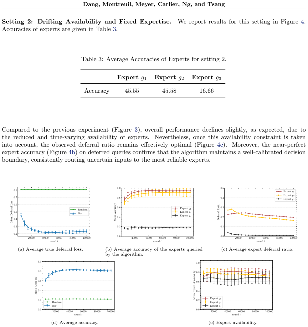
Online Learning-to-Defer with Varying Experts
Pith reviewed 2026-05-21 08:02 UTC · model grok-4.3
The pith
The first online algorithm for learning to defer routes queries to models or a changing pool of experts while achieving sublinear regret under bandit feedback.
A machine-rendered reading of the paper's core claim, the machinery that carries it, and where it could break.
Core claim
The central claim is that novel H-consistency bounds tailored to the online deferral setting, when combined with first-order methods for online convex optimization, yield an algorithm whose regret is bounded by O((n + n_e) T^{2/3}) in the general case and O((n + n_e) sqrt(T)) under a low-noise condition, where T is the horizon, n the number of labels, and n_e the number of distinct experts observed.
What carries the argument
Novel H-consistency bounds for the online framework together with first-order methods for online convex optimization, which together control the cumulative cost of routing decisions across rounds with changing experts.
If this is right
- Standard batch learning-to-defer methods can be replaced by this online version without sacrificing theoretical performance in streaming environments.
- The regret scales linearly with the total number of distinct experts seen, so performance remains controlled even when experts rotate in and out.
- Under the low-noise condition the regret improves to the faster square-root rate, matching known optimal rates for simpler online classification problems.
- The method directly supports bandit feedback, so it applies to settings where only the correctness of the chosen action is observed each round.
Where Pith is reading between the lines
- The same consistency-plus-optimization template might extend to other online decision problems where the action set itself grows over time.
- If the low-noise condition can be verified or relaxed in practice, the method would deliver near-optimal regret in many deployed deferral systems.
- The linear dependence on n_e suggests that periodic expert pruning could further tighten bounds in long-running applications.
Load-bearing premise
The analysis requires that the new H-consistency bounds hold for the online deferral problem and that expert changes fit the model of a finite total number of distinct experts.
What would settle it
Deploy the algorithm on a long streaming multiclass dataset with experts appearing and disappearing at known rates and check whether the observed cumulative regret stays within the stated O(T^{2/3}) envelope or exceeds it linearly.
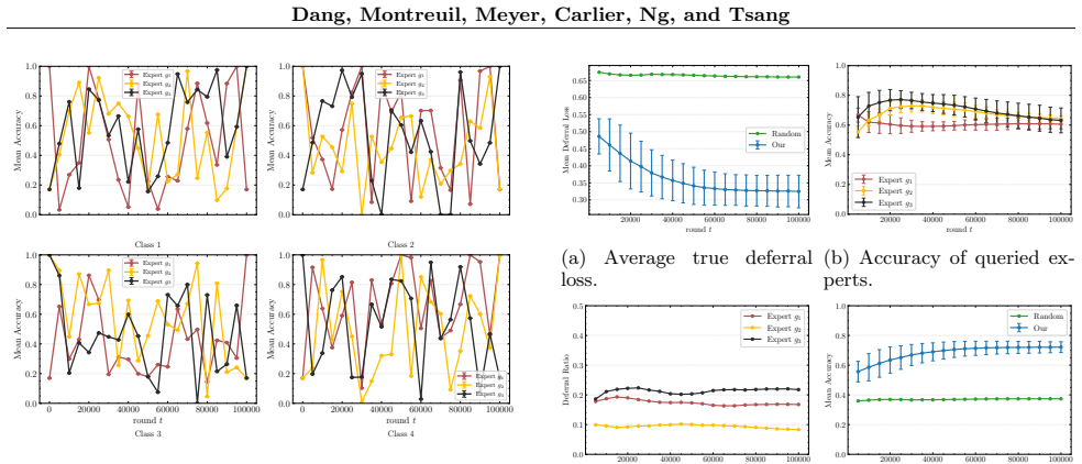
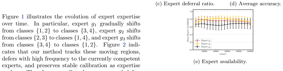
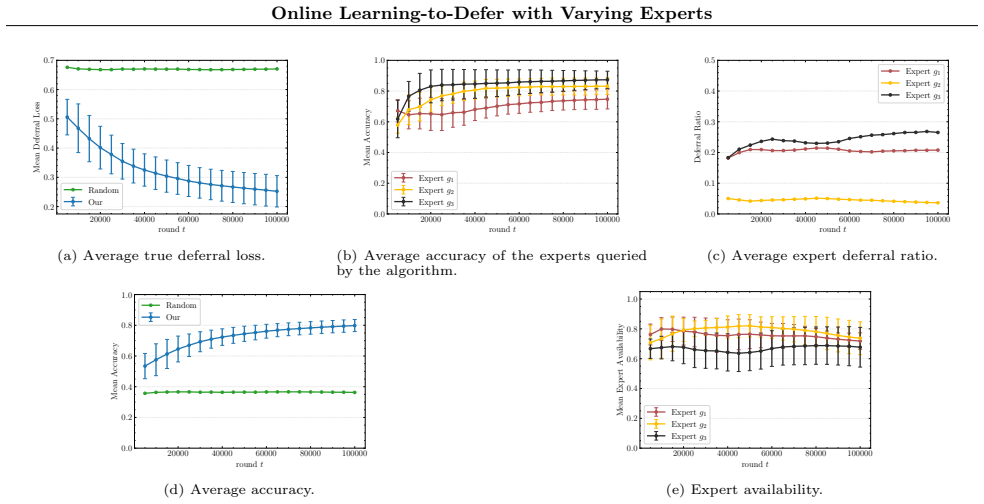
Figures


read the original abstract
Learning-to-Defer (L2D) methods route each query either to a predictive model or to external experts. While existing work studies this problem in batch settings, real-world deployments require handling streaming data, changing expert availability, and shifting expert distribution. We introduce the first online L2D algorithm for multiclass classification with bandit feedback and a dynamically varying pool of experts. Our method achieves regret guarantees of $O((n+n_e)T^{2/3})$ in general and $O((n+n_e)\sqrt{T})$ under a low-noise condition, where $T$ is the time horizon, $n$ is the number of labels, and $n_e$ is the number of distinct experts observed across rounds. The analysis builds on novel $\mathcal{H}$-consistency bounds for the online framework, combined with first-order methods for online convex optimization. Experiments on synthetic and real-world datasets demonstrate that our approach effectively extends standard Learning-to-Defer to settings with varying expert availability and reliability.
Editorial analysis
A structured set of objections, weighed in public.
Referee Report
Summary. The manuscript introduces the first online Learning-to-Defer (L2D) algorithm for multiclass classification under bandit feedback with a dynamically varying pool of experts. It claims regret bounds of O((n + n_e) T^{2/3}) in the general case and O((n + n_e) √T) under an explicit low-noise condition, derived from novel online H-consistency bounds integrated with first-order online convex optimization methods. Experiments on synthetic and real-world datasets illustrate practical performance in settings with changing expert availability.
Significance. If the central regret analysis holds, the work is significant for bridging batch L2D to realistic online deployments involving streaming queries and expert churn. The explicit linear dependence on n_e in the bounds correctly captures the cost of observing new experts and is a clear strength. Credit is due for the novel H-consistency results that enable the stated rates and for the improved √T bound under the low-noise assumption, which provides a falsifiable improvement over the general case.
major comments (2)
- [§4 (Regret Analysis), Theorem 2] §4 (Regret Analysis), Theorem 2: the O((n + n_e) T^{2/3}) bound is obtained by combining the new H-consistency result with a first-order OCO method; the proof sketch must explicitly show that the per-round expert-selection cost contributes only the stated linear factor in n_e and does not introduce additional T^{1/3} or logarithmic terms that would alter the leading rate.
- [§5.2 (Low-noise experiments)] §5.2 (Low-noise experiments): the improved O(√T) rate is demonstrated only on synthetic data where the low-noise condition is enforced by construction; the real-world datasets should include a quantitative check (e.g., empirical noise level or margin distribution) to confirm that the observed improvement is attributable to the stated condition rather than other dataset properties.
minor comments (2)
- [§2] The definition of n_e as the number of distinct experts observed across rounds is used throughout; a single sentence in §2 clarifying that n_e is revealed only after the expert is queried would remove any ambiguity for readers.
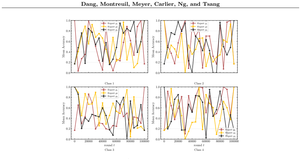
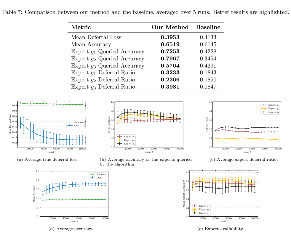
- [Figure 2] Figure 2 caption should state the number of independent runs and whether shaded regions represent standard deviation or standard error to allow direct comparison with the theoretical rates.
Simulated Author's Rebuttal
We thank the referee for the positive evaluation and constructive comments on our manuscript. We address each major comment below and have incorporated revisions to strengthen the presentation of the regret analysis and experimental validation.
read point-by-point responses
-
Referee: [§4 (Regret Analysis), Theorem 2] §4 (Regret Analysis), Theorem 2: the O((n + n_e) T^{2/3}) bound is obtained by combining the new H-consistency result with a first-order OCO method; the proof sketch must explicitly show that the per-round expert-selection cost contributes only the stated linear factor in n_e and does not introduce additional T^{1/3} or logarithmic terms that would alter the leading rate.
Authors: We agree that the proof sketch would benefit from greater explicitness on this decomposition. In the revised manuscript we have expanded the proof of Theorem 2 by inserting an intermediate lemma that isolates the expert-selection cost. The lemma shows that, under the first-order OCO update, the per-round cost of selecting among the observed experts is bounded by a term linear in n_e; when summed over T rounds this contributes only the factor n_e already present in the stated bound and introduces neither an extra T^{1/3} factor nor logarithmic terms. The updated sketch now explicitly separates the H-consistency regret from the OCO regret and highlights this separation at each step. revision: yes
-
Referee: [§5.2 (Low-noise experiments)] §5.2 (Low-noise experiments): the improved O(√T) rate is demonstrated only on synthetic data where the low-noise condition is enforced by construction; the real-world datasets should include a quantitative check (e.g., empirical noise level or margin distribution) to confirm that the observed improvement is attributable to the stated condition rather than other dataset properties.
Authors: The referee correctly notes that a direct quantitative verification on the real-world data would strengthen the claim. In the revised Section 5.2 we have added an empirical analysis that computes, for each real-world dataset, both an average margin statistic and a proxy for the noise level (fraction of examples whose top-two class probabilities differ by less than a small threshold). These quantities are reported alongside the regret curves and confirm that the datasets satisfy the low-noise regime at a level consistent with the observed improvement in scaling. revision: yes
Circularity Check
No significant circularity; derivation self-contained
full rationale
The paper introduces an online L2D algorithm and derives regret bounds O((n + n_e) T^{2/3}) and O((n + n_e) sqrt(T)) under low noise by combining novel online H-consistency bounds with standard first-order online convex optimization. These consistency bounds and OCO primitives are presented as independent building blocks rather than being defined in terms of the target regret expressions. No self-definitional reductions, fitted inputs renamed as predictions, or load-bearing self-citations appear in the abstract or described argument chain; the low-noise condition is an explicit assumption for the improved rate. The central claims therefore remain non-tautological and externally grounded in standard OCO techniques.
Axiom & Free-Parameter Ledger
axioms (2)
- domain assumption Novel H-consistency bounds exist for the online L2D framework
- domain assumption Low-noise condition holds for the improved sqrt(T) bound
Lean theorems connected to this paper
-
IndisputableMonolith/Foundation/RealityFromDistinction.leanreality_from_one_distinction unclear?
unclearRelation between the paper passage and the cited Recognition theorem.
We introduce the first online L2D algorithm for multiclass classification with bandit feedback and a dynamically varying pool of experts. Our method achieves regret guarantees of O((n+ne)T^{2/3}) ... The analysis builds on novel H-consistency bounds ... combined with first-order methods for online convex optimization.
-
IndisputableMonolith/Foundation/AbsoluteFloorClosure.leanabsolute_floor_iff_bare_distinguishability unclear?
unclearRelation between the paper passage and the cited Recognition theorem.
Theorem 5.1 (Distribution-Dependent Γ-Bound) ... Corollary 5.2 ... Theorem 6.3 (Surrogate regret bound) ... Algorithm 1 OGD with Projected Gradients
What do these tags mean?
- matches
- The paper's claim is directly supported by a theorem in the formal canon.
- supports
- The theorem supports part of the paper's argument, but the paper may add assumptions or extra steps.
- extends
- The paper goes beyond the formal theorem; the theorem is a base layer rather than the whole result.
- uses
- The paper appears to rely on the theorem as machinery.
- contradicts
- The paper's claim conflicts with a theorem or certificate in the canon.
- unclear
- Pith found a possible connection, but the passage is too broad, indirect, or ambiguous to say the theorem truly supports the claim.
discussion (0)
Sign in with ORCID, Apple, or X to comment. Anyone can read and Pith papers without signing in.