Gradient-Flow Optimization as Dynamic Random-Effects Inference: Testing and Early Stopping with Applications to Deep Learning

Lin Liu; Minhao Yao; Ruoyu Wang; Xihong Lin; Zhonghua Liu

arxiv: 2605.27991 · v2 · pith:VEHMXFAHnew · submitted 2026-05-27 · 📊 stat.ML · cs.LG

Gradient-Flow Optimization as Dynamic Random-Effects Inference: Testing and Early Stopping with Applications to Deep Learning

Minhao Yao , Ruoyu Wang , Xihong Lin , Lin Liu , Zhonghua Liu This is my paper

Pith reviewed 2026-06-29 10:13 UTC · model grok-4.3

classification 📊 stat.ML cs.LG

keywords gradient flowrandom effectsempirical BayesREMLearly stoppingvariance componentstraining operatordeep learning

0 comments

The pith

Gradient-flow optimization with a fixed positive semidefinite operator is exactly equivalent to empirical-Bayes inference under a random-effects model.

A machine-rendered reading of the paper's core claim, the machinery that carries it, and where it could break.

The paper shows that when fitted values evolve under a time-invariant positive semidefinite training operator, the model output at any training time equals the best linear unbiased predictor from a matching random-effects model. This equivalence makes training duration a variance-component parameter that reallocates variance between residual noise and structured signal. The need to train at all therefore becomes a testable hypothesis on whether signal variance exceeds initialization, while the stopping time becomes a restricted maximum likelihood estimation problem. The resulting early-stopping rule has a spectral reading: it stops when optimized spectral losses are empirically decorrelated from the operator eigenvalues. The framework applies to deep learning models in fixed-kernel regimes and delivers competitive prediction accuracy with less reliance on validation splits.

Core claim

Whenever the fitted value evolves through a time-invariant positive semidefinite training operator, the trained model output at each training time is exactly equivalent to the best linear unbiased predictor, or empirical-Bayes posterior mean, under a corresponding random-effects model. Under this representation, training time becomes a variance-component parameter governing how variance is reallocated from residual noise to structured signal. This turns whether training is needed into a variance-component test for signal beyond initialization and how long to train into restricted maximum likelihood estimation of the training-time variance component, with asymptotic prediction optimality for

What carries the argument

Fixed-operator squared-error gradient flow, which produces outputs identical to the posterior mean trajectory of a dynamic random-effects model whose variance component is the training time.

If this is right

Training duration functions as a variance component that reallocates variance from noise to signal.
Whether training is required reduces to a variance-component test for nonzero signal beyond initialization.
Optimal stopping time is obtained by REML estimation of the training-time variance component.
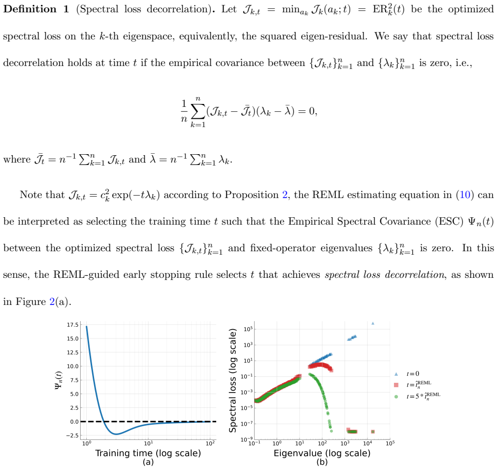
The REML rule selects the time at which spectral losses become decorrelated from the eigenvalues of the training operator.
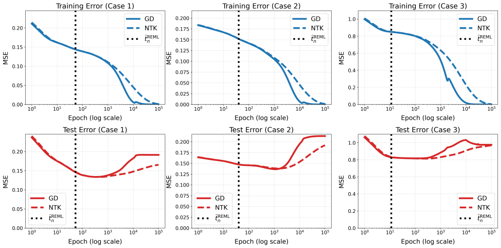
Asymptotic optimality holds for fixed-design in-sample risk and, under kernel regularity, for random-design out-of-sample risk.

Where Pith is reading between the lines

These are editorial extensions of the paper, not claims the author makes directly.

Standard random-effects tools such as prediction intervals or shrinkage estimators could be imported directly into the gradient-flow setting.
If the operator varies slowly the exact equivalence may degrade gracefully, opening a route to approximate inference for more general optimizers.
Running the variance-component test at initialization could detect cases where training adds no value and avoid unnecessary computation.

Load-bearing premise

The training operator stays time-invariant and positive semidefinite throughout the flow, and the model remains inside a fixed-kernel gradient regime.

What would settle it

Compute both the gradient-flow trajectory and the corresponding random-effects BLUP for the same fixed positive semidefinite operator and a chosen training time; any numerical mismatch at that time falsifies the claimed equivalence.

Figures

Figures reproduced from arXiv: 2605.27991 by Lin Liu, Minhao Yao, Ruoyu Wang, Xihong Lin, Zhonghua Liu.

**Figure 2.** Figure 2: (a). Empirical spectral covariance (ESC) Ψ [PITH_FULL_IMAGE:figures/full_fig_p021_2.png] view at source ↗

**Figure 3.** Figure 3: Comparison of gradient descent and NTK gradient flow in numerical experiments. The vertical [PITH_FULL_IMAGE:figures/full_fig_p028_3.png] view at source ↗

**Figure 4.** Figure 4: Training and test MSE curves for LDL, HbA1c, SBP, and BMI. The black dotted line indicates [PITH_FULL_IMAGE:figures/full_fig_p030_4.png] view at source ↗

read the original abstract

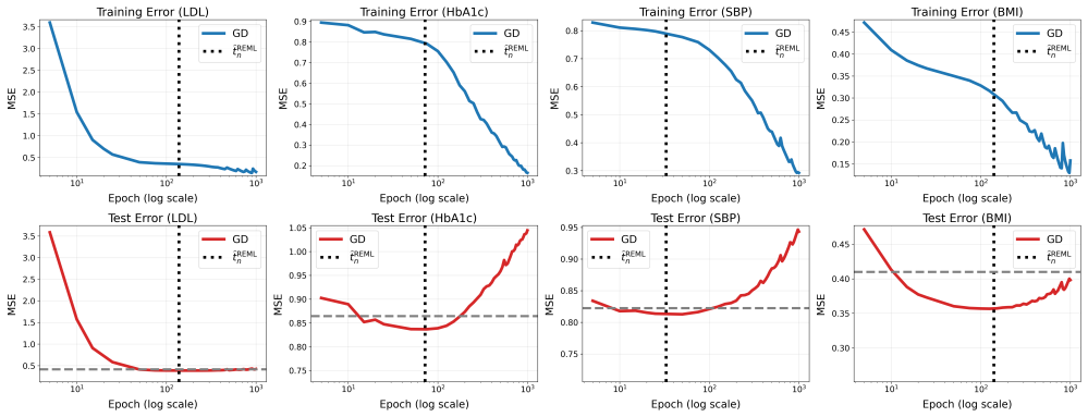
Gradient-flow optimization is usually viewed as an algorithmic procedure for minimizing empirical loss, with training duration selected by validation or heuristic early-stopping rules. We develop a statistical inference framework for the gradient-flow training trajectory itself. The central object is fixed-operator squared-error gradient flow: whenever the fitted value evolves through a time-invariant positive semidefinite training operator, the trained model output at each training time is exactly equivalent to the best linear unbiased predictor, or empirical-Bayes posterior mean, under a corresponding random-effects model. Under this representation, training time becomes a variance-component parameter governing how variance is reallocated from residual noise to structured signal. This turns two basic training decisions into inferential problems. First, whether training is needed is formulated as a variance-component test for signal beyond initialization. Second, how long to train is formulated as restricted maximum likelihood (REML) estimation of the training-time variance component. The resulting REML-guided early stopping rule has a spectral interpretation: it selects the training time at which optimized spectral losses become empirically decorrelated from the eigenvalues of the training operator, yielding an effective degrees-of-freedom measure for the evolving trained model. We establish asymptotic prediction optimality for fixed-design in-sample risk and, under additional kernel regularity conditions, random-design out-of-sample risk. Deep learning models in fixed-kernel gradient regimes provide canonical modern-AI instantiations of the theory. Numerical experiments and a UK Biobank proteomics application show that the proposed inferential approach attains competitive prediction accuracy while reducing the reliance on validation splits and repeated checkpoint evaluation.

Editorial analysis

A structured set of objections, weighed in public.

Desk editor's note, referee report, simulated authors' rebuttal, and a circularity audit. Tearing a paper down is the easy half of reading it; the pith above is the substance, this is the friction.

Desk Editor's Note private letter to a colleague

Gradient flow with a fixed PSD operator is exactly the BLUP from a matching random-effects model, which lets them derive a REML early-stopping rule.

read the letter

The paper shows that whenever the training operator stays constant and positive semidefinite, the gradient-flow trajectory is identical to the empirical-Bayes posterior mean of a random-effects model, with training time as the variance component. From this they obtain a test for whether any training is needed and a REML rule that stops when the spectral losses are decorrelated from the operator eigenvalues.

What is new is the explicit random-effects representation and the resulting REML criterion; the spectral matching and the asymptotic optimality claims for in-sample and (under kernel conditions) out-of-sample risk follow directly once the equivalence is in place. The UK Biobank proteomics example indicates the rule can match validation-based stopping while using less held-out data.

The load-bearing assumption is that the operator remains time-invariant. In most deep-learning settings the effective operator changes, so the exact equivalence holds only in the fixed-kernel regime the authors flag. How well the REML rule performs as an approximation when that assumption is mildly violated is not settled by the abstract. Finite-sample behavior of the variance-component estimator also receives less attention than the asymptotics.

This is for readers who already work at the intersection of optimization, kernel methods, and empirical Bayes. Someone looking for a statistically motivated alternative to validation early stopping in linear or fixed-kernel problems will get the most out of it. The derivation is clean enough and the optimality statements precise enough that it deserves a serious referee.

Referee Report

2 major / 3 minor

Summary. The manuscript claims that gradient-flow optimization through any fixed time-invariant positive semidefinite training operator yields a trajectory that is exactly equivalent to the best linear unbiased predictor (or empirical-Bayes posterior mean) under a matching random-effects model, with training time serving as the variance-component parameter. This representation converts the decisions of whether and how long to train into variance-component testing and REML estimation, respectively; the resulting REML early-stopping rule has a spectral decorrelation interpretation. Asymptotic in-sample and (under kernel regularity) out-of-sample risk optimality are established, with numerical experiments and a UK Biobank proteomics application.

Significance. If the stated equivalence holds, the paper supplies a statistically grounded alternative to validation-based early stopping that directly exploits the spectral structure of the training operator. The exact matching to the BLUP formula, the derivation of an effective-degrees-of-freedom measure from REML, and the asymptotic optimality results constitute the main contributions.

major comments (2)

[§2] §2, Eq. (3)–(7): the central equivalence is asserted to be exact once the operator A is time-invariant and PSD, yet the manuscript does not explicitly verify that the REML estimator of the variance component remains independent of the fitted trajectory after the operator is fixed; a short algebraic check confirming that the profiled likelihood does not re-introduce dependence on the training path would strengthen the claim.
[§5] §5, Theorem 3: the out-of-sample risk optimality result is stated under “additional kernel regularity conditions,” but the precise minimal assumptions (e.g., eigenvalue decay rate or Mercer kernel boundedness) that allow the fixed-design equivalence to carry over to random design are not listed; without them the scope of the optimality guarantee is difficult to assess.

minor comments (3)

The notation for the training operator A and the variance-component parameter τ should be introduced once in §2 and used uniformly thereafter; occasional re-definition in later sections is distracting.
Figure 2 (spectral loss plots) would be clearer if the vertical axis were labeled as the empirical decorrelation measure rather than left as “loss.”
The UK Biobank experiment reports point estimates of prediction accuracy; adding standard errors obtained from the REML information matrix would allow readers to judge whether the reported gains are statistically distinguishable.

Simulated Author's Rebuttal

2 responses · 0 unresolved

We thank the referee for the constructive comments and the recommendation for minor revision. We address each major comment below and will incorporate the suggested clarifications into the revised manuscript.

read point-by-point responses

Referee: [§2] §2, Eq. (3)–(7): the central equivalence is asserted to be exact once the operator A is time-invariant and PSD, yet the manuscript does not explicitly verify that the REML estimator of the variance component remains independent of the fitted trajectory after the operator is fixed; a short algebraic check confirming that the profiled likelihood does not re-introduce dependence on the training path would strengthen the claim.

Authors: We agree that an explicit verification strengthens the claim. Because the operator A is fixed and time-invariant, the profiled REML objective is a function solely of the eigenvalues of A and the response vector y; the equivalence to the BLUP trajectory does not feed back into the likelihood, so the maximizer of the profiled likelihood is independent of any intermediate fitted values along the path. We will add a short algebraic verification (one paragraph or an appendix lemma) confirming that the profiled likelihood depends only on the fixed spectral decomposition of A. revision: yes
Referee: [§5] §5, Theorem 3: the out-of-sample risk optimality result is stated under “additional kernel regularity conditions,” but the precise minimal assumptions (e.g., eigenvalue decay rate or Mercer kernel boundedness) that allow the fixed-design equivalence to carry over to random design are not listed; without them the scope of the optimality guarantee is difficult to assess.

Authors: We accept that the minimal conditions should be stated explicitly rather than left as a reference to “additional kernel regularity.” The required conditions are: (i) the kernel is Mercer and uniformly bounded, and (ii) the eigenvalues of the integral operator decay at a polynomial rate sufficient for the random-design bias term to be controlled by the fixed-design spectral quantities. We will revise the statement of Theorem 3 (and the surrounding paragraph) to list these assumptions explicitly. revision: yes

Circularity Check

0 steps flagged

No significant circularity: equivalence is a direct ODE-to-BLUP derivation

full rationale

The paper's core claim is a mathematical equivalence obtained by solving the linear ODE df/dt = −A(f − y) for constant PSD operator A, yielding the spectral filter (I − exp(−tA)), and matching it to the posterior mean formula of a random-effects model whose variance component is set proportional to t. This is an explicit construction of a corresponding model, not a self-definitional loop or fitted parameter renamed as prediction. No load-bearing self-citation is invoked for the equivalence itself; variance-component tests and REML early stopping are downstream applications of the representation. The derivation remains self-contained against external benchmarks and does not reduce any claimed result to its own inputs by construction.

Axiom & Free-Parameter Ledger

1 free parameters · 2 axioms · 0 invented entities

Only the abstract is available, so the ledger is necessarily incomplete. The central claim rests on the time-invariance and positive-semidefiniteness of the training operator and on the fixed-kernel gradient regime; these appear as domain assumptions rather than derived results.

free parameters (1)

training-time variance component
Treated as the parameter estimated by REML; its value directly determines the stopping time.

axioms (2)

domain assumption The training operator is time-invariant and positive semidefinite.
Invoked to establish the exact equivalence to the random-effects model.
domain assumption Models operate in fixed-kernel gradient regimes.
Required for the deep-learning instantiations of the theory.

pith-pipeline@v0.9.1-grok · 5824 in / 1443 out tokens · 21828 ms · 2026-06-29T10:13:35.876670+00:00 · methodology

discussion (0)

Reference graph

Works this paper leans on

8 extracted references · 2 canonical work pages · 2 internal anchors

[1]

J., Bambrick, J., et al

Abramson, J., Adler, J., Dunger, J., Evans, R., Green, T., Pritzel, A., Ronneberger, O., Willmore, L., Ballard, A. J., Bambrick, J., et al. (2024). Accurate structure prediction of biomolecular interactions with AlphaFold 3.Nature, 630(8016):493–500. Achour, E. M., Malgouyres, F., and Gerchinovitz, S. (2024). The loss landscape of deep linear neural netwo...

2024
[2]

He, K., Zhang, X., Ren, S., and Sun, J

Springer. He, K., Zhang, X., Ren, S., and Sun, J. (2016). Deep residual learning for image recognition. InProceedings of the IEEE conference on computer vision and pattern recognition, pages 770–778. 39 Henderson, C. R. (1975). Best linear unbiased estimation and prediction under a selection model. Biometrics, 31(2):423–447. Jacot, A., Gabriel, F., and Ho...

2016
[3]

There Will Be a Scientific Theory of Deep Learning

42 Rudin, C. (2019). Stop explaining black box machine learning models for high stakes decisions and use interpretable models instead.Nature Machine Intelligence, 1(5):206–215. Ruppert, D., Wand, M. P., and Carroll, R. J. (2003).Semiparametric Regression. Cambridge Series in Statistical and Probabilistic Mathematics. Cambridge University Press, Cambridge ...

work page internal anchor Pith review Pith/arXiv arXiv 2019
[4]

Mining Useful General Data for Low-Resource Domain Adaptation

Cambridge University Press. Wang, P., Liu, H., Liao, Y., Fan, Z., Du, Y., Tang, S., Wang, Y., and Wang, Y. (2025). Selecting auxiliary data via neural tangent kernels for low-resource domains.arXiv preprint arXiv:2511.07380. Woodworth, B., Gunasekar, S., Lee, J. D., Moroshko, E., Savarese, P., Golan, I., Soudry, D., and Srebro, N. (2020). Kernel and rich ...

work page internal anchor Pith review Pith/arXiv arXiv 2025
[5]

The result follows immediately from the mean value theorem

Combining these bounds yields d dt EVn(t) ≤Cn ¯λ for allt≤ ¯λ−1. The result follows immediately from the mean value theorem. S7 Proof of Lemma S3 Proof.Let r=f ⋆(X)−f 0(X),B t := 1 n et¯λ exp(−tH). Then Vn(t) = (r+ε) ⊤Bt(r+ε), and therefore Vn(t)−EV n(t) = 2r⊤Btε+ ε⊤Btε−E[ε ⊤Btε] . Fort≤ ¯λ−1, we have ∥Bt∥op = 1 n max 1≤k≤n et(¯λ−λk) ≤ e n , and ∥Bt∥2 F =...

2013
[6]

59 Define the empirical fixed operator (bT f)(x) = 1 n nX i=1 h(x,x i)f(x i)

by takingrtherein as⌊ √n⌋. 59 Define the empirical fixed operator (bT f)(x) = 1 n nX i=1 h(x,x i)f(x i). The nonzero eigenvalues of bTareλ k/n. More precisely, ifHv k =λ kvk, then the corresponding empirical eigenfunction is bϕk(x) = √nh(x,X)v k/λk, and it satisfies bTbϕk =λ kbϕk/n. At the training covariatesbϕk(xℓ) = √n vkℓ withv kℓ being theℓth componen...

2005
[7]

LetS n :H →R n be the evaluation operatorS nf={f(x 1),

Under Condition S5,r∈ Hand ∥r∥2 H = X k≥1 β2 k µk <∞. LetS n :H →R n be the evaluation operatorS nf={f(x 1), . . . , f(xn)}⊤. ThenH=S nS∗ n withS ∗ n being the adjoint operator ofS n. For eachλ k >0, define bgk =λ −1/2 k S∗ nvk = r λk n bϕk =λ −1/2 k h(·,X)v k. 61 BecauseHv k =λ kvk, we have ⟨bgk,bgj⟩H = v⊤ k Hv jp λkλj =1{k=j}. Thus{bgk}n k=1 is an ortho...

2005
[8]

For anyC >0, let QC ={Q f :f=f 0 +hwith∥h∥ H ≤C}. 65 Under the conditionsE[f 0(x)4]<∞and sup x |h(x,x)|<∞, the function classQ C isP-Donsker according to Example 1.8.5, Theorem 2.6.14, and Lemma 2.6.20 of van der Vaart and Wellner (1996). Therefore, sup q∈QC |(Pn −P X)q|=O p(n−1/2).(S11) In addition, for anyϵ >0, there is someCsuch thatQ bf H btREMLn ∈ Q ...

1996

[1] [1]

J., Bambrick, J., et al

Abramson, J., Adler, J., Dunger, J., Evans, R., Green, T., Pritzel, A., Ronneberger, O., Willmore, L., Ballard, A. J., Bambrick, J., et al. (2024). Accurate structure prediction of biomolecular interactions with AlphaFold 3.Nature, 630(8016):493–500. Achour, E. M., Malgouyres, F., and Gerchinovitz, S. (2024). The loss landscape of deep linear neural netwo...

2024

[2] [2]

He, K., Zhang, X., Ren, S., and Sun, J

Springer. He, K., Zhang, X., Ren, S., and Sun, J. (2016). Deep residual learning for image recognition. InProceedings of the IEEE conference on computer vision and pattern recognition, pages 770–778. 39 Henderson, C. R. (1975). Best linear unbiased estimation and prediction under a selection model. Biometrics, 31(2):423–447. Jacot, A., Gabriel, F., and Ho...

2016

[3] [3]

There Will Be a Scientific Theory of Deep Learning

42 Rudin, C. (2019). Stop explaining black box machine learning models for high stakes decisions and use interpretable models instead.Nature Machine Intelligence, 1(5):206–215. Ruppert, D., Wand, M. P., and Carroll, R. J. (2003).Semiparametric Regression. Cambridge Series in Statistical and Probabilistic Mathematics. Cambridge University Press, Cambridge ...

work page internal anchor Pith review Pith/arXiv arXiv 2019

[4] [4]

Mining Useful General Data for Low-Resource Domain Adaptation

Cambridge University Press. Wang, P., Liu, H., Liao, Y., Fan, Z., Du, Y., Tang, S., Wang, Y., and Wang, Y. (2025). Selecting auxiliary data via neural tangent kernels for low-resource domains.arXiv preprint arXiv:2511.07380. Woodworth, B., Gunasekar, S., Lee, J. D., Moroshko, E., Savarese, P., Golan, I., Soudry, D., and Srebro, N. (2020). Kernel and rich ...

work page internal anchor Pith review Pith/arXiv arXiv 2025

[5] [5]

The result follows immediately from the mean value theorem

Combining these bounds yields d dt EVn(t) ≤Cn ¯λ for allt≤ ¯λ−1. The result follows immediately from the mean value theorem. S7 Proof of Lemma S3 Proof.Let r=f ⋆(X)−f 0(X),B t := 1 n et¯λ exp(−tH). Then Vn(t) = (r+ε) ⊤Bt(r+ε), and therefore Vn(t)−EV n(t) = 2r⊤Btε+ ε⊤Btε−E[ε ⊤Btε] . Fort≤ ¯λ−1, we have ∥Bt∥op = 1 n max 1≤k≤n et(¯λ−λk) ≤ e n , and ∥Bt∥2 F =...

2013

[6] [6]

59 Define the empirical fixed operator (bT f)(x) = 1 n nX i=1 h(x,x i)f(x i)

by takingrtherein as⌊ √n⌋. 59 Define the empirical fixed operator (bT f)(x) = 1 n nX i=1 h(x,x i)f(x i). The nonzero eigenvalues of bTareλ k/n. More precisely, ifHv k =λ kvk, then the corresponding empirical eigenfunction is bϕk(x) = √nh(x,X)v k/λk, and it satisfies bTbϕk =λ kbϕk/n. At the training covariatesbϕk(xℓ) = √n vkℓ withv kℓ being theℓth componen...

2005

[7] [7]

LetS n :H →R n be the evaluation operatorS nf={f(x 1),

Under Condition S5,r∈ Hand ∥r∥2 H = X k≥1 β2 k µk <∞. LetS n :H →R n be the evaluation operatorS nf={f(x 1), . . . , f(xn)}⊤. ThenH=S nS∗ n withS ∗ n being the adjoint operator ofS n. For eachλ k >0, define bgk =λ −1/2 k S∗ nvk = r λk n bϕk =λ −1/2 k h(·,X)v k. 61 BecauseHv k =λ kvk, we have ⟨bgk,bgj⟩H = v⊤ k Hv jp λkλj =1{k=j}. Thus{bgk}n k=1 is an ortho...

2005

[8] [8]

For anyC >0, let QC ={Q f :f=f 0 +hwith∥h∥ H ≤C}. 65 Under the conditionsE[f 0(x)4]<∞and sup x |h(x,x)|<∞, the function classQ C isP-Donsker according to Example 1.8.5, Theorem 2.6.14, and Lemma 2.6.20 of van der Vaart and Wellner (1996). Therefore, sup q∈QC |(Pn −P X)q|=O p(n−1/2).(S11) In addition, for anyϵ >0, there is someCsuch thatQ bf H btREMLn ∈ Q ...

1996