SubsurfaceGen: Procedural Generation of Field-Scale Earth Models and Seismic Data
Pith reviewed 2026-06-29 08:51 UTC · model grok-4.3
The pith
SubsurfaceGen generates field-scale 3D velocity models and paired seismic data to train and test ML methods for full waveform inversion.
A machine-rendered reading of the paper's core claim, the machinery that carries it, and where it could break.
Core claim
SubsurfaceGen produces 3D velocity models spanning 10 km x 10 km laterally and 6.19 km deep at 10 m resolution, together with 5 s wavefields and 8 s shot gathers. The released dataset contains 4,276 2D velocity slices from 42 models in six geological settings, supporting tests of wavefield prediction and end-to-end velocity inversion with out-of-distribution evaluation on held-out settings.
What carries the argument
SubsurfaceGen, a GPU-accelerated procedural generator that builds physically realistic 3D velocity models and corresponding seismic data at field scale.
If this is right
- Neural operators for wavefield prediction and encoder-decoders for velocity inversion can be evaluated at spatial and temporal scales matching actual field applications.
- Holding out entire geological settings enables direct measurement of out-of-distribution performance in subsurface imaging tasks.
- Paired velocity and seismic data allow quantitative assessment of end-to-end inversion accuracy at 10 m resolution over 10 km extents.
- The dataset construction from six distinct geological settings supports targeted testing for applications such as carbon sequestration and hydrocarbon exploration.
Where Pith is reading between the lines
- If the generated models capture essential geological features, the same generator could supply training data for related geophysical tasks such as travel-time tomography.
- Larger volumes of paired data from this approach might allow systematic study of how model size and geological complexity interact in learned inversion methods.
- The procedural nature of the generator suggests it could be extended to produce time-lapse or anisotropic models for testing more advanced inversion scenarios.
Load-bearing premise
The procedurally generated models are realistic and diverse enough that training and testing on them reveals the actual limitations ML models will face with real field data.
What would settle it
If models trained on the SubsurfaceGen dataset show the same performance and failure modes on real seismic surveys as models trained only on smaller existing datasets like Marmousi or OpenFWI, the claim that the new data impacts ML-based FWI would not hold.
Figures







read the original abstract
Full waveform inversion (FWI) is the gold standard for subsurface imaging, with applications from carbon sequestration to energy and mineral exploration to earthquake hazard assessment. Machine learning approaches to FWI need field-scale, geologically diverse, and physically realistic training data, but existing resources such as Marmousi, SEAM, and OpenFWI fall short on spatial extent, temporal extent, geological diversity, and physical realism. We address these limitations with SubsurfaceGen, a GPU-accelerated generator for 3D velocity models and seismic data. Along with SubsurfaceGen, we release a paired dataset of 4,276 2D velocity slices, 5 s wavefields, and 8 s shot gathers drawn from 42 realistic, field-scale 3D velocity models, each spanning 10 km x 10 km laterally and 6.19 km deep at 10 m resolution. The dataset spans six geological settings -- four built with SubsurfaceGen and two drawn from prior sources -- relevant for carbon sequestration and hydrocarbon exploration. We use this dataset to evaluate neural operators on wavefield prediction and encoder-decoders on end-to-end velocity inversion, holding out one geological setting for out-of-distribution testing. These experiments surface failure modes at field-scale and demonstrate how SubsurfaceGen and the associated dataset can impact ML-based FWI.
Editorial analysis
A structured set of objections, weighed in public.
Referee Report
Summary. The paper introduces SubsurfaceGen, a GPU-accelerated procedural generator for creating 3D velocity models and seismic data at field scale. It releases a paired dataset consisting of 4,276 2D velocity slices, 5 s wavefields, and 8 s shot gathers drawn from 42 realistic 3D models (each 10 km x 10 km x 6.19 km at 10 m resolution) spanning six geological settings relevant to carbon sequestration and hydrocarbon exploration (four generated with SubsurfaceGen, two from prior sources). The authors evaluate neural operators on wavefield prediction and encoder-decoders on end-to-end velocity inversion, with one geological setting held out for out-of-distribution testing, claiming that the experiments surface failure modes at field scale.
Significance. If the generated models prove sufficiently realistic and diverse, the work supplies a much-needed large-scale resource for ML-based FWI that addresses documented shortcomings of Marmousi, SEAM, and OpenFWI in spatial extent, temporal extent, and geological variety. The explicit release of the generator, code, and paired dataset constitutes a concrete, reusable contribution that can support reproducible research and systematic identification of ML limitations in realistic settings.
major comments (2)
- [Dataset construction] Dataset construction paragraph: the central claim that the procedurally generated models are 'realistic' and capable of surfacing meaningful field-scale failure modes rests on an unverified assumption of physical and geological fidelity; the manuscript provides no quantitative validation such as velocity histograms, spatial autocorrelation statistics, or direct comparison against real field surveys.
- [Evaluation setup] Evaluation setup: the OOD experiments hold out one geological setting, but the text does not specify which setting is held out nor demonstrate that the held-out geology differs in a manner that genuinely tests generalization rather than merely presenting a new realization of similar geology.
minor comments (2)
- [Abstract] Abstract: the phrases '5 s wavefields' and '8 s shot gathers' are ambiguous; clarify whether these refer to simulation duration, recording length, or another quantity.
- [Introduction] Introduction: the discussion of limitations of Marmousi, SEAM, and OpenFWI would benefit from explicit numerical comparisons (e.g., lateral extent, depth, number of distinct geological regimes) rather than qualitative statements.
Simulated Author's Rebuttal
We thank the referee for the positive assessment and constructive feedback. We address each major comment below.
read point-by-point responses
-
Referee: [Dataset construction] Dataset construction paragraph: the central claim that the procedurally generated models are 'realistic' and capable of surfacing meaningful field-scale failure modes rests on an unverified assumption of physical and geological fidelity; the manuscript provides no quantitative validation such as velocity histograms, spatial autocorrelation statistics, or direct comparison against real field surveys.
Authors: We acknowledge that the manuscript does not include quantitative statistical comparisons such as velocity histograms, spatial autocorrelation, or direct comparisons to real field surveys. Realism claims rest on the use of established procedural methods for the six geological settings. In revision we will add velocity histograms and basic statistical summaries of the generated models to support the claims. revision: yes
-
Referee: [Evaluation setup] Evaluation setup: the OOD experiments hold out one geological setting, but the text does not specify which setting is held out nor demonstrate that the held-out geology differs in a manner that genuinely tests generalization rather than merely presenting a new realization of similar geology.
Authors: We agree the held-out setting should be named and the geological distinctions motivating the OOD test should be made explicit. In the revised manuscript we will identify the held-out setting and add a brief description of its distinguishing features relative to the training settings. revision: yes
Circularity Check
No significant circularity
full rationale
This is a methods and data-release paper describing a procedural generator for velocity models and seismic data, plus a released dataset and illustrative ML experiments. No mathematical derivations, predictions, or uniqueness claims are present that could reduce by construction to fitted parameters or self-citations. The OOD hold-out uses independent geological settings, and the central deliverable (generator + data) does not rely on any load-bearing step that loops back to its own inputs.
Axiom & Free-Parameter Ledger
Reference graph
Works this paper leans on
-
[1]
Penobscot Dataset: Fostering Machine Learning Development for Seismic Interpretation
Lais Baroni, Reinaldo Mozart Silva, Rodrigo S. Ferreira, Daniel Civitarese, Daniela Szwarcman, and Emilio Vital Brazil. Penobscot dataset: Fostering machine learning development for seismic interpretation.arXiv preprint arXiv:1903.12060,
work page internal anchor Pith review Pith/arXiv arXiv 1903
-
[2]
arXiv preprint arXiv:2404.09556 (2024) 12, 17, 19, 26, 27, 28, 29, 30, 31
arXiv:2404.09556. Martin P. A. Jackson and Michael R. Hudec.Salt Tectonics: Principles and Practice. Cambridge University Press,
-
[3]
Wave-equation migration velocity analysis
Paul Sava and Biondo Biondi. Wave-equation migration velocity analysis. I. Theory.Geophysical Prospecting, 52(6):593–606, 2004a. Paul Sava and Biondo Biondi. Wave-equation migration velocity analysis. II. Subsalt imaging examples.Geophysical Prospecting, 52(6):607–623, 2004b. Alan Schiemenz and Heiner Igel. Accelerated 3-D full-waveform inversion using si...
1970
-
[4]
Netherlands Dataset: A New Public Dataset for Machine Learning in Seismic Interpretation
Reinaldo Mozart Silva, Lais Baroni, Rodrigo S. Ferreira, Daniel Civitarese, Daniela Szwarcman, and Emilio Vital Brazil. Netherlands dataset: A new public dataset for machine learning in seismic interpretation.arXiv preprint arXiv:1904.00770. Society of Exploration Geophysicists. SEAM Open Data. https://seg.org/SEAM/open-data/,
work page internal anchor Pith review Pith/arXiv arXiv 1904
-
[5]
Deep Dix: Enhancing interval velocity model estima- tion through adversarial regularization
Joseph Stitt, Robert Clapp, and Biondo Biondi. Deep Dix: Enhancing interval velocity model estima- tion through adversarial regularization. InThird International Meeting for Applied Geoscience & Energy (SEG IMAGE 2023), Technical Program Expanded Abstracts, pages 108–112,
2023
-
[6]
A Related Work We discuss related work along three threads: datasets used to train and evaluate ML-based FWI (Section A.1), machine learning methods for seismic modeling and inversion (Section A.2), and software tools for building velocity models (Section A.3). A.1 Datasets for ML-based FWI Marmousi [Versteeg, 1994, Martin et al., 2006], SEAM [Fehler and ...
1994
-
[7]
Jin et al
A second line of work learns the inverse map from shot gathers directly to velocity models using neural networks [Araya-Polo et al., 2018, Yang and Ma, 2019, Wu and Lin, 2020, Zhang and Lin, 2020, Wang et al., 2023b]. Jin et al
2018
-
[8]
Only Farris et al
scales this approach to 408,000 samples, but is restricted to the small spatial extent of OpenFWI (0.7 km). Only Farris et al. [2023], Farris
2023
-
[9]
A third line of work uses generative models trained on velocity models as data-driven priors for FWI [Mosser et al., 2020, Stitt et al., 2023, Wang et al., 2023a, Stitt et al., 2025]; SubsurfaceGen provides a distribution of geologically plausible velocity models required for training these priors. A.3 Model Building Tools Structural geomodeling tools lik...
2020
-
[10]
sinusoidal
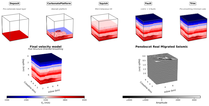
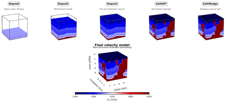
adds a sedimentary package with interbeds (thin layers of contrasting velocity) on top of a model. Interbed boundaries are 2D surfaces sampled from a 3D simplex noise field (a smooth, spatially correlated random field); each bed is assigned a single Gaussian-drawn velocity with a global depth gradient added across the slab, and an additional 3D simplex no...
2009
-
[11]
The goal is not to simulate salt mechanics directly, but to create the common seismic appearance of sediment layers bending, draping, or onlapping near salt bodies
deforms the sediment column in the neighborhood of salt bodies (produced by SaltSDT) to generate flanking onlap and drape geometries consistent with the halokinetic sequence framework of Giles and Rowan [2012]. The goal is not to simulate salt mechanics directly, but to create the common seismic appearance of sediment layers bending, draping, or onlapping...
2012
-
[12]
"] then builds # a Config. Pattern: Module(Config(**cfg[...])).apply(m)↪→ cfg = load_yaml(
implements structure-oriented smoothing [Hale, 2009]. The goal is to smooth the velocity volume anisotropically: strongly along the local bed direction, weakly across it. The operator estimates local orientation from a structure tensor built from Sobel-filtered gradients of V , then computes an eigendecomposition of the smoothed structure tensor to constr...
2009
-
[13]
top” and a “bot
at 4500 m/s, placed at depth fractions [0.15,0.60] , with a correlation length of 0.7 in each axis on the GRF perturbing the body boundary. The SaltWedge module then deforms the surrounding sediment with a combination of a Gaussian weight in distance to the nearest vertical flank, a radial drag weight raised to the 1.8 power, a depth-dependent taper, and ...
2012
-
[14]
Per-stage timings use time.perf_counter() bracketed by torch.cuda.synchronize() on the GPU run
Methodology.Each (setting, device) pair runs as a new Python subprocess. Per-stage timings use time.perf_counter() bracketed by torch.cuda.synchronize() on the GPU run. GPU utilization and memory usage are sampled 10 times per second, i.e., at 10 Hz. Per-setting totals.Table 7 stacks the wall-time breakdown alongside peak GPU memory and peak CPU memory. W...
1907
-
[15]
Splits.Per-setting train slice counts: F3 10×97 = 970 , GoM 10×73 = 730 , faulted-complex 5×145 = 725 , salt-canopy 4×181 = 724 , SEAM 12×79 = 947
All extracted 2D slices inherit this normalization, so the 4,276 shipped slices satisfy vp ∈[1500,5000] m/s without further per-slice modification, consistent with the dispersion (Section E.3.1) and CFL (Section E.3.2) constraints derived below. Splits.Per-setting train slice counts: F3 10×97 = 970 , GoM 10×73 = 730 , faulted-complex 5×145 = 725 , salt-ca...
2019
-
[16]
After filtering, the amplitude of the wavelet depends sensitively on the passband, so we apply a two-step normalization for numerical stability and physical scaling
The peak frequencies are f0 ∈ {4.50,5.75,7.50,10.25,14.00} Hz for the five bands respectively, and each wavelet is centered att0 = 1/f0. After filtering, the amplitude of the wavelet depends sensitively on the passband, so we apply a two-step normalization for numerical stability and physical scaling. We first divide by theℓ2 norm of the filtered signal, ...
2019
-
[17]
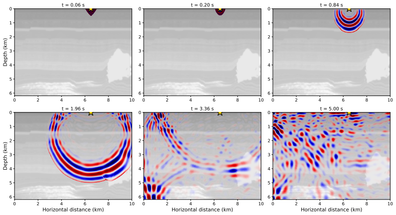
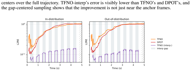
The task is to predict the wavefield (5 s of acoustic propagation at 3–6 Hz) given the velocity slice and a binary source mask; we evaluate three operators: TFNO 32 (chunked autoregressive forward prediction), TFNO-interp (anchor-bounded interior prediction), and DPOT (transformer with adaptive Fourier mixing). F.1 Task setup and preprocessing Tensor shap...
2023
-
[18]
giving higher priority to earlier timesteps will reduce the overall propagation of errors and enhance training stability
formulate the same hypothesis for autoregressive neural operators on 1D PDEs (“giving higher priority to earlier timesteps will reduce the overall propagation of errors and enhance training stability”). Our schedule applies the practice statically: w(t) decays linearly from wstart = 1.0 at t= 0tow end = 0.5att=T out −1, scaling the gradient signal in prop...
2024
-
[19]
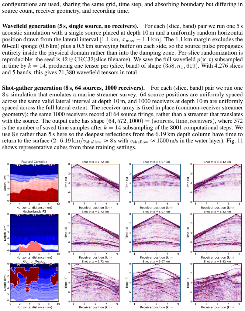
The task is to map a 3D shot-gather cube (produced by 8 s of acoustic propagation at 3–25 Hz) to a 2Dv p(x)velocity model. 36 G.1 Task setup and preprocessing Tensor shapes.The input is a 3D shot-gather cube of shape (nshots, ntime, nreceivers) = (64,572,1000) , presented to the network as (B,1,64,572,1000) , where B is the batchsize. The output is a 2D v...
2022
discussion (0)
Sign in with ORCID, Apple, or X to comment. Anyone can read and Pith papers without signing in.