First-Order Trajectory Matching: Fast Ensemble Predictions of Chaotic, Turbulent, Stochastic Systems
Pith reviewed 2026-06-27 13:46 UTC · model grok-4.3
The pith
First-order trajectory matching learns probability current velocity directly from data to match ensemble averages in stochastic systems.
A machine-rendered reading of the paper's core claim, the machinery that carries it, and where it could break.
Core claim
FTM matches the symmetric first-order motion of trajectories to learn the probability current velocity, whose flow preserves time marginals to match ensemble averages, while capturing current-like trajectory quantities such as fluxes, circulations, and barrier-crossing currents; the method learns this velocity directly from trajectories and avoids drift, diffusion, and score estimation.
What carries the argument
Symmetric first-order motion matching, which learns the probability current velocity from trajectory data to preserve time marginals.
If this is right
- FTM supplies trajectory-aware ensemble predictions for chaotic, turbulent, and stochastic systems.
- Predictions are obtained at low deterministic-rollout cost after training.
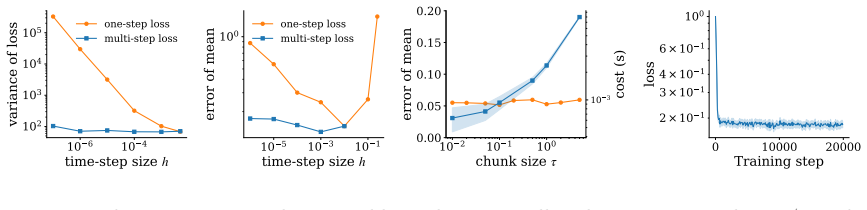
- The one-step simulation-free loss remains stable when temporal resolution and sample size are balanced.
- FTM captures fluxes, circulations, and barrier-crossing currents in addition to marginal statistics.
Where Pith is reading between the lines
- The approach may scale to high-dimensional real-world systems where full Monte Carlo ensembles remain prohibitive.
- FTM outputs could serve as cheap initial conditions or constraints for hybrid physics-ML models.
- Systems with known analytic probability currents offer direct tests of whether first-order matching recovers the exact velocity field.
Load-bearing premise
Matching the symmetric first-order motion of trajectories is sufficient to recover the probability current velocity whose flow preserves time marginals.
What would settle it
A direct comparison on a stochastic system where FTM ensemble averages diverge from independent Monte Carlo ground truth when higher-order trajectory effects dominate.
Figures


read the original abstract
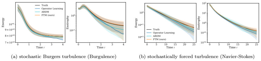
We introduce First-Order Trajectory Matching (FTM), a surrogate-modeling method that learns the first-order local transport of probability mass from trajectories of stochastic systems. By matching the symmetric first-order motion of trajectories, FTM learns the probability current velocity, whose flow preserves time marginals to match ensemble averages, while also capturing current-like trajectory quantities such as fluxes, circulations, and barrier-crossing currents. FTM learns the current velocity directly from trajectories, avoiding drift, diffusion, and score estimation. Our stability analysis separates discretization error from sampling variance and shows that the one-step simulation-free FTM loss is stable when temporal resolution and sample size are properly balanced. Across stochastic dynamical systems and PDE examples, we empirically demonstrate that FTM provides trajectory-aware ensemble predictions at low, deterministic-rollout cost.
Editorial analysis
A structured set of objections, weighed in public.
Referee Report
Summary. The manuscript introduces First-Order Trajectory Matching (FTM), a surrogate-modeling approach that learns the probability current velocity directly from trajectories of stochastic systems by matching symmetric first-order motions. The central claim is that the resulting deterministic flow preserves time marginals to match ensemble averages, while also capturing fluxes and circulations, at low rollout cost without estimating drift, diffusion, or scores. A stability analysis separates discretization error from sampling variance for the one-step simulation-free loss, and empirical results are shown on stochastic dynamical systems and PDEs.
Significance. If the central claim holds, FTM offers a computationally efficient alternative for ensemble predictions in chaotic, turbulent, and stochastic regimes by replacing stochastic rollouts with deterministic integration of a learned velocity field. The separation of error sources in the stability analysis and the direct use of trajectory data without auxiliary estimations are positive features that could impact surrogate modeling for high-dimensional systems.
major comments (2)
- [Abstract] Abstract (FTM definition paragraph): the assertion that matching symmetric first-order trajectory motions yields a velocity field v whose deterministic flow exactly satisfies the continuity equation for the time-evolving marginals p(t) is stated without an explicit weak-form derivation (e.g., equivalence of the loss to ∫(v−J/p)·∇ϕ p dx=0 for test functions ϕ). This equivalence is load-bearing for the claim that deterministic rollouts match ensemble averages over long horizons.
- [Stability analysis] Stability analysis: the separation of discretization error from sampling variance is presented for the one-step loss, but it is unclear whether the analysis extends to the preservation of marginals under iterated deterministic integration in turbulent regimes where higher-order correlations may affect long-horizon behavior.
minor comments (2)
- [Abstract] The abstract mentions empirical demonstrations but does not name the specific stochastic systems or PDE examples; adding one sentence would improve clarity.
- Notation for the probability current velocity and the symmetric first-order motion should be introduced with a short equation in the main text for readers unfamiliar with the continuity-equation context.
Simulated Author's Rebuttal
We are grateful to the referee for their detailed review and constructive feedback. We address each major comment below.
read point-by-point responses
-
Referee: [Abstract] Abstract (FTM definition paragraph): the assertion that matching symmetric first-order trajectory motions yields a velocity field v whose deterministic flow exactly satisfies the continuity equation for the time-evolving marginals p(t) is stated without an explicit weak-form derivation (e.g., equivalence of the loss to ∫(v−J/p)·∇ϕ p dx=0 for test functions ϕ). This equivalence is load-bearing for the claim that deterministic rollouts match ensemble averages over long horizons.
Authors: We agree that an explicit reference to the weak-form equivalence would strengthen the abstract. The main text establishes that the FTM loss is equivalent to a weak-form minimization aligning the learned velocity with the probability current (via integration against test functions), which ensures the deterministic flow satisfies the continuity equation for the marginals. In the revised manuscript we will add a concise statement of this equivalence to the abstract. revision: yes
-
Referee: [Stability analysis] Stability analysis: the separation of discretization error from sampling variance is presented for the one-step loss, but it is unclear whether the analysis extends to the preservation of marginals under iterated deterministic integration in turbulent regimes where higher-order correlations may affect long-horizon behavior.
Authors: The stability analysis deliberately targets the one-step loss to isolate discretization error from sampling variance. Preservation of marginals under iterated integration follows directly from the velocity approximating the probability current, whose flow satisfies the continuity equation by construction; higher-order correlations are not required for this first-order transport property. Our empirical results on long-horizon predictions in chaotic and turbulent regimes provide supporting evidence. We will expand the discussion section to clarify the scope of the analysis and its relation to multi-step behavior. revision: partial
Circularity Check
No significant circularity; derivation self-contained
full rationale
The abstract and description present FTM as learning the probability current velocity via one-step trajectory matching, with stability analysis separating discretization and sampling effects, and empirical validation on systems. No quoted equations or self-citations reduce the central claim (that matching symmetric first-order motions yields a flow preserving marginals) to a definitional identity, fitted input renamed as prediction, or load-bearing self-citation chain. The method is described as simulation-free and directly from trajectories without the target result presupposed in the loss. This meets the default expectation of a non-circular paper.
Axiom & Free-Parameter Ledger
axioms (1)
- domain assumption Matching the symmetric first-order motion of trajectories learns the probability current velocity whose flow preserves time marginals.
Reference graph
Works this paper leans on
-
[1]
Albergo, N
M. Albergo, N. M. Boffi, and E. Vanden-Eijnden. Stochastic interpolants: A unifying framework for flows and diffusions.Journal of Machine Learning Research, 26(209):1–80, 2025
2025
-
[2]
M. S. Albergo and E. Vanden-Eijnden. Building normalizing flows with stochastic interpolants.arXiv preprint arXiv:2209.15571, 2022
Pith/arXiv arXiv 2022
-
[3]
B. D. Anderson. Reverse-time diffusion equation models.Stochastic Processes and their Applications, 12(3):313–326, 1982
1982
-
[4]
Bartosh, D
G. Bartosh, D. Vetrov, and C. A. Naesseth. SDE Matching: Scalable and Simulation- Free Training of Latent Stochastic Differential Equations. InProceedings of the 42nd International Conference on Machine Learning, volume 267 ofProceedings of Machine Learning Research, pages 3054–3070. PMLR, 2025
2025
- [5]
-
[6]
Berman, T
J. Berman, T. Blickhan, and B. Peherstorfer. Parametric Model Reduction of Mean-Field and Stochastic Systems via Higher-Order Action Matching. InAdvances in Neural Information Processing Systems, 2024. 14
2024
-
[7]
Blickhan, J
T. Blickhan, J. Berman, A. Stuart, and B. Peherstorfer. DICE: Discrete inverse continuity equation for learning population dynamics, 2025
2025
-
[8]
N. M. Boffi, M. S. Albergo, and E. Vanden-Eijnden. How to build a consistency model: Learning flow maps via self-distillation. InThe Thirty-ninth Annual Conference on Neural Information Processing Systems, 2025
2025
-
[9]
N. M. Boffi and E. Vanden-Eijnden. Probability flow solution of the Fokker–Planck equation.Machine Learning: Science and Technology, 4(3):035012, jul 2023
2023
-
[10]
N. M. Boffi and E. Vanden-Eijnden. Deep learning probability flows and entropy production rates in active matter.Proceedings of the National Academy of Sciences, 121(25):e2318106121, 2024
2024
-
[11]
N. M. Boffi and E. Vanden-Eijnden. Model-Free Learning of Probability Flows: Eluci- dating the Nonequilibrium Dynamics of Flocking.Phys. Rev. Lett., 135:238301, Dec 2025
2025
-
[12]
Boninsegna, F
L. Boninsegna, F. Nüske, and C. Clementi. Sparse learning of stochastic dynamical equations.The Journal of chemical physics, 148(24), 2018
2018
-
[13]
S. L. Brunton, B. R. Noack, andP. Koumoutsakos. Machine Learning forFluid Mechanics. Annual Review of Fluid Mechanics, 52(Volume 52, 2020):477–508, 2020
2020
-
[14]
ProximalOptimalTransport Modeling of Population Dynamics.arXiv preprint arXiv:2106.06345, 2022
C.Bunne, L.Meng-Papaxanthos, A.Krause, andM.Cuturi. ProximalOptimalTransport Modeling of Population Dynamics.arXiv preprint arXiv:2106.06345, 2022
arXiv 2022
-
[15]
S. Chen, S. Chewi, H. Lee, Y. Li, J. Lu, and A. Salim. The probability flow ODE is provably fast.Advances in Neural Information Processing Systems, 36:68552–68575, 2023
2023
-
[16]
Y. Chen, M. Goldstein, M. Hua, M. S. Albergo, N. M. Boffi, and E. Vanden-Eijnden. Probabilistic Forecasting with Stochastic Interpolants and Föllmer Processes. InPro- ceedings of the 41st International Conference on Machine Learning, volume 235 of Proceedings of Machine Learning Research, pages 6728–6756. PMLR, 21–27 Jul 2024
2024
-
[17]
Chetrite and K
R. Chetrite and K. Gawędzki. Eulerian and Lagrangian pictures of non-equilibrium diffusions.Journal of Statistical Physics, 137(5):890–916, 2009
2009
-
[18]
Comte and V
F. Comte and V. Genon-Catalot. Nonparametric drift estimation for i.i.d. paths of stochastic differential equations.The Annals of Statistics, 48(6):3336 – 3365, 2020
2020
-
[19]
Course and P
K. Course and P. B. Nair. Amortized Reparametrization: Efficient and Scalable Variational Inference for Latent SDEs. InAdvances in Neural Information Processing Systems, volume 36, 2023
2023
-
[20]
B. Das and S. K. Manikandan. Localizing entropy production along non-equilibrium trajectories.arXiv preprint arXiv:2503.20427, 2025
Pith/arXiv arXiv 2025
-
[21]
M. Deng, H. Li, T. Li, Y. Du, and K. He. Generative Modeling via Drifting, 2026. 15
2026
-
[22]
Dresdner, D
G. Dresdner, D. Kochkov, P. Norgaard, L. Zepeda-Núñez, J. A. Smith, M. P. Brenner, and S. Hoyer. Learning to correct spectral methods for simulating turbulent flows. 2022
2022
-
[23]
Dridi, L
N. Dridi, L. Drumetz, and R. Fablet. Learning stochastic dynamical systems with neural networks mimicking the Euler–Maruyama scheme. In2021 29th European Signal Processing Conference (EUSIPCO), pages 1990–1994, Dublin, Ireland, Aug. 2021. IEEE
1990
-
[24]
Frishman and P
A. Frishman and P. Ronceray. Learning Force Fields from Stochastic Trajectories.Phys. Rev. X, 10:021009, Apr 2020
2020
-
[25]
K. Fukumizu, T. Suzuki, N. Isobe, K. Oko, and M. Koyama. Flow matching achieves almost minimax optimal convergence.arXiv preprint arXiv:2405.20879, 2024
arXiv 2024
-
[26]
Z. Geng, M. Deng, X. Bai, J. Z. Kolter, and K. He. Mean Flows for One-step Generative Modeling. InThe Thirty-ninth Annual Conference on Neural Information Processing Systems, 2025
2025
-
[27]
U. G. Haussmann and E. Pardoux. Time Reversal of Diffusions.The Annals of Probability, 14(4):1188–1205, Oct 1986
1986
-
[28]
J. Ho, A. Jain, and P. Abbeel. Denoising diffusion probabilistic models. InAdvances in Neural Information Processing Systems, volume 33, 2020
2020
-
[29]
Jiang, P
R. Jiang, P. Y. Lu, E. Orlova, and R. Willett. Training neural operators to preserve invariant measures of chaotic attractors. InThirty-seventh Conference on Neural Information Processing Systems, 2023
2023
-
[30]
G. E. Karniadakis, I. G. Kevrekidis, L. Lu, P. Perdikaris, S. Wang, and L. Yang. Physics-informed machine learning.Nature Reviews Physics, 3(6):422–440, Jun 2021
2021
-
[31]
Kidger, J
P. Kidger, J. Foster, X. Li, and T. Lyons. Efficient and Accurate Gradients for Neural SDEs. InAdvances in Neural Information Processing Systems, volume 34, pages 18747– 18761, 2021
2021
-
[32]
P. E. Kloeden and E. Platen.Numerical Solution of Stochastic Differential Equations. Stochastic Modelling and Applied Probability. Springer, Berlin, Heidelberg, 1 edition,
-
[33]
Springer-Verlag Berlin Heidelberg (1992); eBook ISBN 978-3-662-12616-5 (2013 reprint)
1992
-
[34]
Kochkov, J
D. Kochkov, J. A. Smith, A. Alieva, Q. Wang, M. P. Brenner, and S. Hoyer. Machine learning–accelerated computational fluid dynamics.Proceedings of the National Academy of Sciences, 118(21), 2021
2021
-
[35]
Kohl, L.-W
G. Kohl, L.-W. Chen, and N. Thuerey. Benchmarking autoregressive conditional diffusion models for turbulent flow simulation.Neural Networks, 199:108641, 2026
2026
-
[36]
J. Li, J. M. Horowitz, T. R. Gingrich, and N. Fakhri. Quantifying dissipation using fluctuating currents.Nature communications, 10(1):1666, 2019. 16
2019
-
[37]
Li, T.-K
X. Li, T.-K. L. Wong, R. T. Q. Chen, and D. Duvenaud. Scalable Gradients for Stochastic Differential Equations. InProceedings of the Twenty Third International Conference on Artificial Intelligence and Statistics, volume 108 ofProceedings of Machine Learning Research, pages 3870–3882. PMLR, 2020
2020
-
[38]
Z. Li, N. Kovachki, K. Azizzadenesheli, B. liu, K. Bhattacharya, A. Stuart, and A. Anand- kumar. Fourier Neural Operator for Parametric Partial Differential Equations. In International Conference on Learning Representations, 2021
2021
-
[39]
Lipman, R
Y. Lipman, R. T. Q. Chen, H. Ben-Hamu, M. Nickel, and M. Le. Flow matching for gen- erative modeling. InThe Eleventh International Conference on Learning Representations, 2023
2023
-
[40]
L. Lu, P. Jin, G. Pang, Z. Zhang, and G. E. Karniadakis. Learning nonlinear operators via DeepONet based on the universal approximation theorem of operators.Nature Machine Intelligence, 3(3):218–229, Mar 2021
2021
-
[41]
J. Lyu, K. J. Ray, and J. P. Crutchfield. Learning Stochastic Thermodynamics Directly from Correlation and Trajectory-Fluctuation Currents.arXiv, 2504.19007, 2025
arXiv 2025
-
[42]
Maoutsa, S
D. Maoutsa, S. Reich, and M. Opper. Interacting Particle Solutions of Fokker–Planck Equations Through Gradient–Log–Density Estimation.Entropy, 22(8), 2020
2020
-
[43]
Molinaro, S
R. Molinaro, S. Lanthaler, B. Raonić, T. Rohner, V. Armegioiu, S. Simonis, D. Grund, Y. Ramic, Z. Y. Wan, F. Sha, S. Mishra, and L. Zepeda-Núñez. Generative AI for fast and accurate statistical computation of fluids. 2025
2025
-
[44]
K. Na, J. Lee, S.-Y. Yun, and S. Lim. Probability-flow ODE in infinite-dimensional function spaces.arXiv preprint arXiv:2503.10219, 2025
arXiv 2025
-
[45]
Neklyudov, R
K. Neklyudov, R. Brekelmans, D. Severo, and A. Makhzani. Action Matching: Learning Stochastic Dynamics from Samples. InProceedings of the 40th International Conference on Machine Learning, volume 202 ofProceedings of Machine Learning Research, pages 25858–25889. PMLR, 2023
2023
-
[46]
Nelson.Dynamical theories of Brownian motion
E. Nelson.Dynamical theories of Brownian motion. Princeton University Press, 1967
1967
-
[47]
J. N. Nielsen, H. Madsen, and P. C. Young. Parameter estimation in stochastic differential equations: an overview.Annual Reviews in Control, 24:83–94, 2000
2000
-
[48]
Otness, A
K. Otness, A. Gjoka, J. Bruna, D. Panozzo, B. Peherstorfer, T. Schneider, and D. Zorin. An extensible benchmark suite for learning to simulate physical systems. InThirty-fifth Conference on Neural Information Processing Systems Datasets and Benchmarks Track (Round 1), 2021
2021
-
[49]
G. A. Pavliotis.Stochastic Processes and Applications: Diffusion Processes, the Fokker- Planck and Langevin Equations, volume 60 ofTexts in Applied Mathematics. Springer New York, New York, NY, 2014. 17
2014
-
[50]
On certain relations between classical statistics and quantum mechanics
L. Peliti and P. Muratore-Ginanneschi. R. Fürth’s 1933 paper “On certain relations between classical statistics and quantum mechanics” [“Über einige Beziehungen zwischen klassischer Statistik und Quantenmechanik”, Zeitschrift für Physik, 81 143–162].The European Physical Journal H, 48(1):4, May 2023
1933
-
[51]
Reiterer, C
P. Reiterer, C. Lainscsek, F. Schürrer, C. Letellier, and J. Maquet. A nine-dimensional Lorenz system to study high-dimensional chaos.Journal of Physics A: Mathematical and General, 31(34):7121, aug 1998
1998
-
[52]
Rey-Bellet and K
L. Rey-Bellet and K. Spiliopoulos. Irreversible Langevin samplers and variance reduction: a large deviations approach.Nonlinearity, 28(7):2081–2103, 2015
2081
-
[53]
Ryder, A
T. Ryder, A. Golightly, A. S. McGough, and D. Prangle. Black-Box Variational Inference for Stochastic Differential Equations. InProceedings of the 35th International Conference on Machine Learning, volume 80 ofProceedings of Machine Learning Research, pages 4423–4432. PMLR, 2018
2018
-
[54]
Sanderse, P
B. Sanderse, P. Stinis, R. Maulik, and S. E. Ahmed. Scientific machine learning for closure models in multiscale problems: A review.Foundations of Data Science, 7(1):298–337, 2025
2025
-
[55]
U. Seifert. Stochastic thermodynamics, fluctuation theorems and molecular machines. Reports on progress in physics, 75(12):126001, 2012
2012
-
[56]
Y. Song, P. Dhariwal, M. Chen, and I. Sutskever. Consistency models.International conference on machine learning, 2023
2023
-
[57]
Y. Song, J. Sohl-Dickstein, D. P. Kingma, A. Kumar, S. Ermon, and B. Poole. Score- Based Generative Modeling through Stochastic Differential Equations. InInternational Conference on Learning Representations, 2021
2021
-
[58]
Stachenfeld, D
K. Stachenfeld, D. B. Fielding, D. Kochkov, M. Cranmer, T. Pfaff, J. Godwin, C. Cui, S. Ho, P. Battaglia, and A. Sanchez-Gonzalez. Learned Coarse Models for Efficient Turbulence Simulation. InInternational Conference on Learning Representations (ICLR 2021), 2021
2021
-
[59]
Terpin, N
A. Terpin, N. Lanzetti, M. Gadea, and F. Dörfler. Learning Diffusion at Lightspeed. In Advances in Neural Information Processing Systems, 2024
2024
-
[60]
A. Tong, J. Huang, G. Wolf, D. van Dijk, and S. Krishnaswamy. TrajectoryNet: A Dynamic Optimal Transport Network for Modeling Cellular Dynamics.arXiv preprint arXiv:2002.04461, 2020
arXiv 2002
-
[61]
Tsimpos, D
P. Tsimpos, D. Sharp, and Y. Marzouk. One-Shot Generative Flows: Existence and Obstructions, 2026
2026
-
[62]
B. Tzen and M. Raginsky. Neural Stochastic Differential Equations: Deep Latent Gaussian Models in the Diffusion Limit.arXiv preprint arXiv:1905.09883, 2019. 18
arXiv 1905
-
[63]
Zhang, Y
X. Zhang, Y. Pu, Y. Kawamura, A. Loza, Y. Bengio, D. L. Shung, and A. Tong. Trajectory Flow Matching with Applications to Clinical Time Series Modeling. In Advances in Neural Information Processing Systems, volume 37, pages 107198–107224, 2024
2024
-
[64]
L. Zhou, S. Ermon, and J. Song. Inductive Moment Matching.arXiv preprint arXiv:2503.07565, 2025. Appendix A. Illustrative examples, and gauge freedom for global mass transport We first specify the SDE toy example shown in Figure 1 in the main text via Example 1. Example1.We consider a statistically stationary, rotating Ornstein–Uhlenbeck process in d= 2di...
arXiv 2025
-
[65]
This probability current corresponds to sample paths of(18) circulating in the same direction, while preserving their time marginal distribution
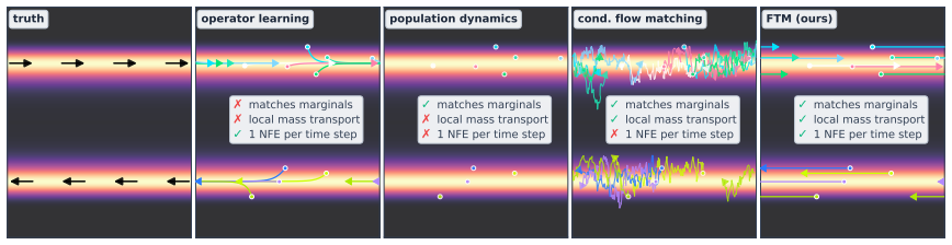
truth:We show the constant marginal distributionρ(t) ≡ρ ∞ of the process onR2 as a heatmap, with white arrows indicating the direction of the analytically known probability current velocityv(x) = ΩRx from (7), which circulates counterclockwise forΩ > 0. This probability current corresponds to sample paths of(18) circulating in the same direction, while pr...
-
[66]
Learning only the drift, and solving the ODEd dt ˆx(t) = b(ˆx(t))at inference, leads to trajectories that spiral inwards and collapse onto the mean0ofρ∞ at large t
operator learning:The target for operator learning is the drift vector fieldb in (18) via (4). Learning only the drift, and solving the ODEd dt ˆx(t) = b(ˆx(t))at inference, leads to trajectories that spiral inwards and collapse onto the mean0ofρ∞ at large t. Hence, this does not preserve the correct time marginals. 19
-
[67]
population dynamics:The main goal of population dynamics is to match the correct time marginals, which are stationary here. These methods typically assume that onlyunpairedsamples from X(t)at different times t are available, without trajectory information (which, as we argue in the present work, is actually available in many problems and useful to train w...
-
[68]
In the figure, we hence show sample paths of the SDE(18) generated using the Euler–Maruyama method
conditional flow matching:Conditional flow matching methods are capable of reproducing the correct transition law ofX(t + h) |X (t)of the SDE(18). In the figure, we hence show sample paths of the SDE(18) generated using the Euler–Maruyama method. By construction, these will have the correct time marginalsρ(t) ≡ρ ∞, and circulate counterclockwise according...
-
[69]
orthogonal component
FTM:Here, we integrate the ODE d dt ˆx(t) = v(t,ˆx(t)), which preserves the time marginals, can be done at low computational cost, and the resulting pure circulation at constant radius mimics the behavior of true sample paths of (18). In order to illustrate and contextualize these points further, it is useful to provide a slightly more abstract view on Ex...
-
[70]
1 τ Z t+τ t ∥vθ(s, X(s))∥2 2ds 2# | {z } ≤2V 4 + 8Et∼U([0,T−τ]),ω∼P
the current velocityvis a gradient field, v(t, x) =−∇U(t, x)− σ(t)2 2 ∇logρ(t, x) =−∇ U(t, x) + σ(t)2 2 logρ(t, x) . 2.vis the unique minimizer of the kinetic energy functional K(u) := Z T 0 Z Rd ρ(t, x)∥u(t, x)∥2 2 dxdt, among all velocity fieldsusatisfying the continuity equation ∂tρ+∇ ·(ρu) = 0. Hence, in this setting, the probability current velocityv...
-
[71]
Using the Cauchy-Schwarz inequality for integrals and the uniform bounds∥b(t, x)∥2 ≤ bmax and∥v θ(t, x)∥2 ≤V, we get Eω " 1 τ Z t+τ t ⟨vθ(s, Xω(s)), b(s, Xω(s))⟩ds 2# ≤V 2b2 max
-
[72]
Using the Itô isometry and the boundΣ(t) =A(t)A(t)⊤ ⪯σ maxId, we have Eω " 1 τ Z t+τ t ⟨vθ(s, Xω(s)), A(s)dWω(s)⟩ 2# = 1 τ 2 Eω Z t+τ t ⟨vθ(s, Xω(s)),Σ(s)v θ(s, Xω(s))⟩ds ≤ 1 τ 2 Eω Z t+τ t σmax∥vθ(s, Xω(s))∥2 2ds ≤ σmaxV 2 τ
-
[73]
C.3 Variance of the one-step FTM loss ash↓0, and relation to symmetric differences In this section, we discuss the one-step FTM objective(16) from the main text
Lastly, using the assumptionCdiv = supt,x 1 2 |Tr[Σ(t)∇v θ(t, x)]|<∞, we have Eω " 1 2τ Z t+τ t Tr [Σ(s)∇vθ(s, Xω(s))] ds 2# ≤C 2 div , which completes the proof since all of these bounds are independent oft∼ U ([0, T−τ ]). C.3 Variance of the one-step FTM loss ash↓0, and relation to symmetric differences In this section, we discuss the one-step FTM objec...
-
[74]
For fixedθ∈R p, the velocity fieldvθ is bounded in the sense that there existsV > 0 such that ∥vθ(t, x)∥2 ≤Vfor allt∈[0, T], x∈R d
-
[75]
We formulate this as an assumption here for brevity, but such a bound can be derived by using standard weak Taylor arguments for the forward and reverse process [32]
The symmetric increment (6) is first-order accurate in the sense ∥vh(t, x)−v(t, x)∥ 2 ≤Ch ,(25) for a constantC > 0and all t∈ [h, T−h ], x∈R d. We formulate this as an assumption here for brevity, but such a bound can be derived by using standard weak Taylor arguments for the forward and reverse process [32]. We have the following upper bound on the mean-...
discussion (0)
Sign in with ORCID, Apple, or X to comment. Anyone can read and Pith papers without signing in.