From Brewing to Resolution: Tracing the Internal Lifecycle of Code Reasoning in LLMs
Pith reviewed 2026-06-27 01:04 UTC · model grok-4.3
The pith
LLMs brew code answers in a stable early phase before diverging into four resolution outcomes with only 41.5 percent success overall.
A machine-rendered reading of the paper's core claim, the machinery that carries it, and where it could break.
Core claim
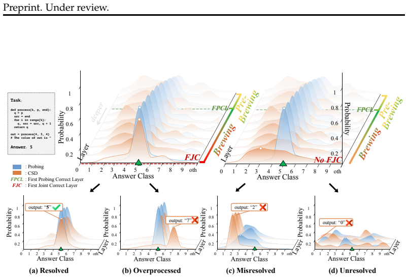
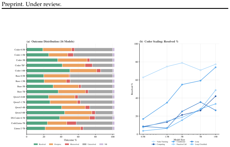
In decoder-only Transformers, code reasoning proceeds through an early brewing phase where the answer is linearly recoverable many layers before it becomes self-decodable, after which the model enters one of four resolution outcomes—Resolved, Overprocessed, Misresolved, or Unresolved—with an overall Resolved rate of 41.5 percent and sharp drops such as function-call resolution falling from 61.1 percent to 2.5 percent as call depth increases from one to three.
What carries the argument
The dual diagnostic framework of layer-wise linear probing paired with Context-Stripped Decoding that locates the brewing phase and assigns each instance to one of the four resolution outcomes.
If this is right
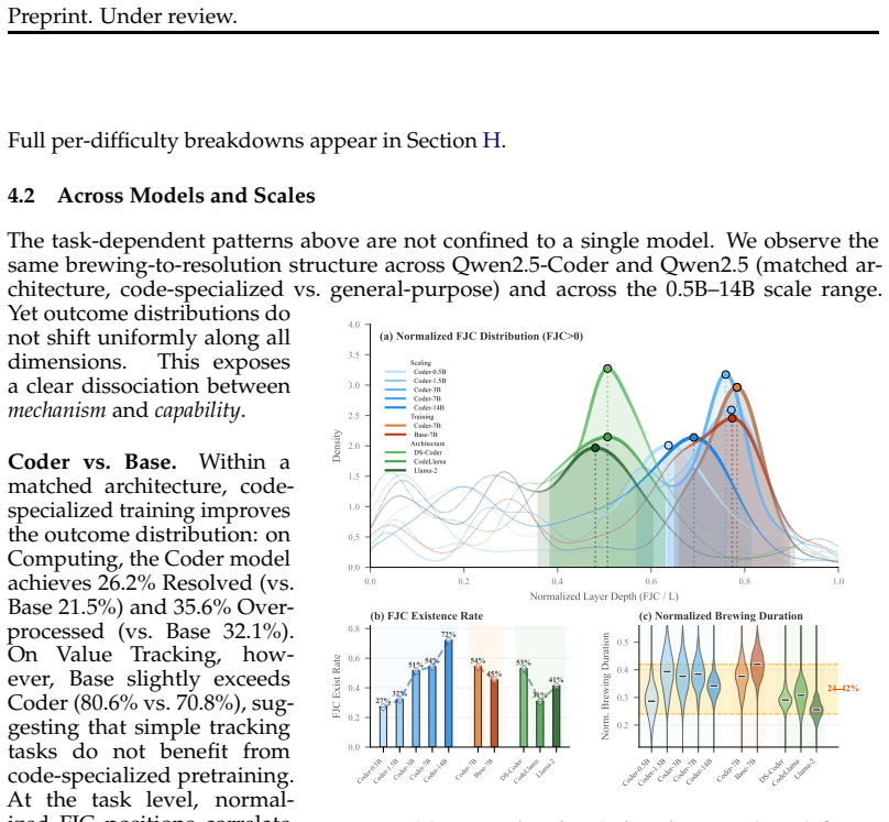
- The brewing scaffold occupies a stable 24-42 percent of layers across all sixteen tested models regardless of architecture or scale.
- Resolution success covaries with model capability, scale, and training data rather than with the presence of the scaffold itself.
- Task structure creates specific bottlenecks, such as the sharp decline in function-call resolution with increased nesting depth.
- Every task family distributes mass across all four resolution outcomes rather than concentrating in Resolved or Unresolved alone.
Where Pith is reading between the lines
- The same probing-plus-CSD method could be applied to non-code reasoning tasks to test whether a comparable brewing scaffold appears.
- If the brewing phase can be lengthened or stabilized through training interventions, resolution rates might increase without changing model size.
- Outcome labels could serve as a finer-grained training signal than binary correctness to reduce overprocessing or misresolution.
- Layer-specific interventions during the brewing window might shift more instances into the Resolved category.
Load-bearing premise
Layer-wise linear probing combined with Context-Stripped Decoding can reliably mark the brewing phase and separate the four outcomes without the measured durations or distributions depending on post-hoc threshold or classifier choices.
What would settle it
Re-running the same traces with a different linear probe architecture or altered CSD stopping criterion that produces substantially different brewing durations or outcome fractions would falsify the claim that the lifecycle is stably identified.
Figures


read the original abstract
Standard accuracy metrics cannot explain why LLMs handle variable tracking but fail on semantically equivalent loops. We study an internal lifecycle of code reasoning in which models first brew the answer, making it linearly recoverable many layers before it becomes self-decodable, and then diverge into one of four resolution outcomes: Resolved, Overprocessed, Misresolved, or Unresolved. Understanding this lifecycle matters because similar task accuracies can mask fundamentally different failure modes that surface-level evaluation cannot detect. We introduce a dual diagnostic framework pairing layer-wise linear probing with Context-Stripped Decoding (CSD) and apply it to six code-reasoning task families across 16 models spanning Qwen, Llama, and DeepSeek architectures. All four outcomes carry substantial mass in every task family: overall Resolved is only 41.5%, with multiple tasks below 30%. Controlled sweeps over structure, depth, and operators expose task-specific failure bottlenecks: Function Call Resolved plunges from 61.1% to 2.5% as call depth increases from one to three. Across architectures and scales, the brewing scaffold remains stable, with normalized brewing duration 24-42% across all 16 models, while resolution success varies with capability. This indicates that the scaffold is a stable empirical regularity across the tested decoder-only Transformer families, whereas resolution success covaries with capability, scale, and training. Code: https://github.com/euyis1019/llm-brewing
Editorial analysis
A structured set of objections, weighed in public.
Referee Report
Summary. The manuscript claims that LLMs follow an internal 'brewing' lifecycle for code reasoning: answers first become linearly recoverable via layer-wise probing many layers before becoming self-decodable via Context-Stripped Decoding (CSD), after which models diverge into one of four resolution outcomes (Resolved, Overprocessed, Misresolved, Unresolved). Applying the dual framework to six task families across 16 models (Qwen, Llama, DeepSeek), it reports a stable normalized brewing duration of 24-42% across all models, overall Resolved rate of 41.5% (with multiple tasks below 30%), and task-specific bottlenecks such as Function Call Resolved dropping from 61.1% to 2.5% with increasing call depth. Resolution success varies with capability while the brewing scaffold does not.
Significance. If the diagnostics prove robust, the work would provide a useful decomposition of reasoning failures that surface accuracy metrics miss, with the stable brewing duration across architectures offering a potential empirical regularity for decoder-only Transformers. The public code release is a positive for reproducibility.
major comments (2)
- [Dual diagnostic framework] Dual diagnostic framework (as introduced in the abstract and applied throughout): the reported stability of normalized brewing duration (24-42%) and the 41.5% Resolved figure are defined via linear probing recoverability and CSD self-decodability, yet no sensitivity analysis is reported on probing accuracy cutoffs, classifier splits, or context-stripping depth. This is load-bearing for the central claim that the scaffold is an intrinsic regularity rather than an artifact of post-hoc thresholds.
- [Outcome distributions and task sweeps] Results on outcome distributions (abstract and task-family sweeps): the four resolution outcomes are classified using the same probing/CSD diagnostics, so any threshold dependence directly affects the claim that all four carry substantial mass in every task family and the task-specific failure bottlenecks (e.g., Function Call depth effect). No error bars, controls for probing classifier choice, or alternative threshold definitions are mentioned.
minor comments (2)
- [Abstract] The abstract states consistent results across 16 models but does not specify how outcomes are thresholded or whether statistical controls were applied; adding this detail would improve clarity without altering the core claims.
- [Framework definition] Minor notation: 'normalized brewing duration' is used without an explicit equation in the provided summary; defining it formally would aid readers.
Simulated Author's Rebuttal
We thank the referee for the constructive feedback, which identifies key areas for strengthening the empirical robustness of the dual diagnostic framework. We address the major comments point by point below.
read point-by-point responses
-
Referee: [Dual diagnostic framework] Dual diagnostic framework (as introduced in the abstract and applied throughout): the reported stability of normalized brewing duration (24-42%) and the 41.5% Resolved figure are defined via linear probing recoverability and CSD self-decodability, yet no sensitivity analysis is reported on probing accuracy cutoffs, classifier splits, or context-stripping depth. This is load-bearing for the central claim that the scaffold is an intrinsic regularity rather than an artifact of post-hoc thresholds.
Authors: We agree that the lack of reported sensitivity analysis on probing accuracy cutoffs, classifier splits, and context-stripping depth is a limitation for establishing the brewing scaffold as an intrinsic regularity. While the consistency of the 24-42% normalized brewing duration across 16 models from three distinct families provides supporting evidence against pure artifact, we will add dedicated sensitivity analyses in the revision. These will vary the probing accuracy threshold (e.g., 70%, 80%, 90%), use multiple classifier train/test splits and random seeds, and test alternative CSD stripping depths, reporting the resulting range for normalized brewing duration and Resolved rates. revision: yes
-
Referee: [Outcome distributions and task sweeps] Results on outcome distributions (abstract and task-family sweeps): the four resolution outcomes are classified using the same probing/CSD diagnostics, so any threshold dependence directly affects the claim that all four carry substantial mass in every task family and the task-specific failure bottlenecks (e.g., Function Call depth effect). No error bars, controls for probing classifier choice, or alternative threshold definitions are mentioned.
Authors: We concur that the outcome distributions, including the overall 41.5% Resolved rate and task-specific patterns such as the Function Call depth effect, are sensitive to the same diagnostic thresholds. We will revise the manuscript to include error bars from multiple classifier training seeds, controls using alternative probing classifiers (e.g., logistic regression versus small MLPs), and results under varied threshold definitions. These will be added to the task-family sweeps and outcome distribution figures to better substantiate the reported masses and bottlenecks. revision: yes
Circularity Check
No significant circularity; measurements are operationally defined via independent diagnostics
full rationale
The paper defines brewing duration as the normalized gap between linear recoverability (via layer-wise probing) and self-decodability (via CSD), with the four resolution outcomes likewise labeled by these same external procedures. These are standard diagnostic techniques applied uniformly, not parameters fitted to the target statistics or defined in terms of the reported percentages (24-42% brewing, 41.5% Resolved). No equations reduce claims to tautologies, no self-citations bear the central premise, and no ansatz or uniqueness theorem is smuggled in. The stability finding is an empirical regularity observed across 16 models using consistent, non-self-referential methods.
Axiom & Free-Parameter Ledger
free parameters (2)
- outcome classification thresholds
- normalized brewing duration cutoff
axioms (2)
- domain assumption Linear probing on hidden states can detect when an answer is recoverable before the model can decode it
- domain assumption Context-Stripped Decoding isolates the resolution phase without altering the underlying representations
Reference graph
Works this paper leans on
-
[1]
SWE-bench: Can Language Models Resolve Real-World GitHub Issues?
URLhttps://arxiv.org/abs/2310.06770. Saurav Kadavath, Tom Conerly, Amanda Askell, Tom Henighan, Dawn Drain, Ethan Perez, Nicholas Schiefer, Zac Hatfield-Dodds, Nova DasSarma, Eli Tyre, Zhili Feng, Sandipan Kundu, Jacob Steinhardt, Chris Olah, Sam McCandlish, Dario Amodei, Jackson Kernion, Andy Jones, Jared Kaplan, Tom Brown, Catherine Olsson, and Sam Bowm...
work page internal anchor Pith review Pith/arXiv arXiv doi:10.1145/512927.512945 2022
-
[2]
Value Tracking vs. Function Call— identical structural skeletons (nested function calls with optional distractors), but Value Tracking passes values directly without transformation while Function Call applies arithmetic at every layer. This contrast isolates the cost of intra-function computation from cross-boundary tracking
-
[3]
Two-step addition: 1+3+2=6. Answer:6. Most complex(structure=accumulator,steps=4,operators=add_mul): defscore_items(items, threshold):
Loop vs. Loop Unrolled— identical numerical computations, but Loop uses ex- plicitfor-loop syntax whereas Loop Unrolled writes each iteration as a sequential statement. This contrast isolates the cognitive cost of loop syntax (iteration variable, range, termination condition) from the cost of the underlying computation itself. C.1 Task Definitions Table 2...
-
[4]
Candidates exceeding this range are rejected and resampled (up to 200 attempts per slot)
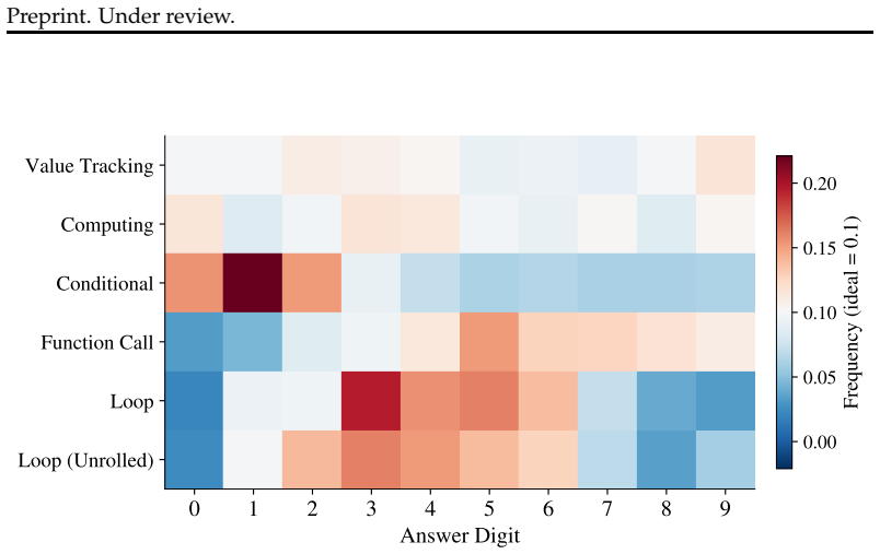
Range filtering.Each generator ensures the computed answer satisfies 0 ≤ answer≤ 9 before accepting a sample. Candidates exceeding this range are rejected and resampled (up to 200 attempts per slot)
-
[5]
Similarly, Function Call’scontainer_relay mechanism uses small positive increments ( {1, 2}) to keep cumulative sums in range
Operand constraints.For tasks involving multiplication (the add_mul operator set in Computing), multiplicative operands are restricted to {0, 1, 2, 3} to prevent re- sults from exceeding single-digit range. Similarly, Function Call’scontainer_relay mechanism uses small positive increments ( {1, 2}) to keep cumulative sums in range
-
[6]
Randomized starting points.Each sample independently draws random initial values, operator choices, branch conditions, and identifier names.random.seed() is set once per task generation, ensuring reproducibility while allowing diverse answer distributions across configurations
-
[7]
availability has not yet onset
Execution verification.Every generated sample is verified by executing its code in a sandboxed Python environment (restricted builtins, no I/O), confirming that the runtime result matches the declared answer. Samples failing this check are flagged and excluded. Thevalidate_and_save routine reports per-task answer distributions and per-dimension breakdowns...
2024
-
[8]
Extract the hidden state hℓ S at the last token position at layerℓ
Run the source prompt S through the full model. Extract the hidden state hℓ S at the last token position at layerℓ
-
[9]
At layer ℓ, replace the last-token hidden state in the target run: ˜hℓ T ←h ℓ S
Construct a separate forward pass with T. At layer ℓ, replace the last-token hidden state in the target run: ˜hℓ T ←h ℓ S. (8) 29 Preprint. Under review
-
[10]
probe-correct,
Continue the target forward pass from layer ℓ+1 through L−1, applying the re- maining transformer blocks, LayerNorm, and the unembedding matrix Wu. The attention context for all subsequent layers is restricted toT. This yields patched logits: zℓ patch =W u ◦LN◦F L−1 ◦ · · · ◦F ℓ+1( ˜hℓ T). Step 3: Baseline subtraction.Running T alone (without patching) pr...
2024
-
[11]
Only 2.7% (39 samples) areNO_BREWINGcases that happen to be correct
FPCL nearly always exists(97.3%): the probe reads the correct answer at some layers, confirming that the information is encoded in a linearly readable form in the hidden states. Only 2.7% (39 samples) areNO_BREWINGcases that happen to be correct
-
[12]
CSD final-layer accuracy is only 28.4%: despite the model producing the correct final output, CSD can decode the answer at the last layer for only about one quarter of samples. For the majority of unexpectedly correct samples, the answer informa- tion is encoded in acontext-dependentform—requiring the full context for decoding, which hidden-state injectio...
-
[13]
decoupled
The “decoupled” pattern(97.3% − 27.1% = 70.2%): a large fraction of samples exhibit probing-readable but CSD-unreadable answer information, forming a per- sistent “information available but not self-decodable” state. This is mechanistically consistent with the core FPCL<FJC gap, except that for these samples the gap never closes. Conclusion.H3 is supporte...
2024
-
[14]
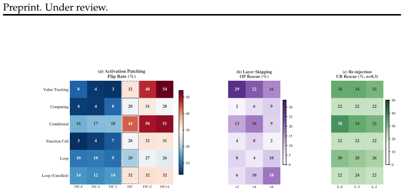
The mean pre-to- FJC jump is+21.2 pp
Universal FJC transition.All six tasks exhibit a sharp flip-rate jump at offset 0, confirming that FJC is a causally meaningful transition point across task categories. The mean pre-to- FJC jump is+21.2 pp
-
[15]
continued rise.Value Tracking and Conditional continue to rise at +2 and +4, indicating ongoing signal consolidation
Post-FJC plateau vs. continued rise.Value Tracking and Conditional continue to rise at +2 and +4, indicating ongoing signal consolidation. Computing and Function Call plateau near FJC, consistent with a single discrete transition
-
[16]
In contrast, Function Call and Computing have very low pre-FJC rates ( ≤ 8%), indicating answer dependence on non-local computations not yet complete before FJC
Pre-FJC background.Conditional shows elevated pre-FJC flip rates (16–18%), suggesting partial answer leakage before FJC—consistent with branching conditions that can be locally evaluated before full computation completes. In contrast, Function Call and Computing have very low pre-FJC rates ( ≤ 8%), indicating answer dependence on non-local computations no...
-
[17]
Loop-unrolled.The unrolled variant shows a larger FJC jump ( +18.3 vs
Loop vs. Loop-unrolled.The unrolled variant shows a larger FJC jump ( +18.3 vs. +9.8 pp) and higher absolute flip rates, suggesting that explicit loop syntax in the non- 42 Preprint. Under review. unrolled version forces more distributed cross-layer processing, reducing causal concen- tration at any single layer. F.6 Localizing the Overprocessing Rewrite:...
-
[18]
ˆȷint ≈(H early C −H tail C )/ ln|D|
Entropy conservation. ˆȷint ≈(H early C −H tail C )/ ln|D| . The information flux integral is essentially the difference between early and tail entropy, which can be fully reconstructed from endpoints
-
[19]
Over such short sequences, Varℓ∈W (H ℓ C) carries almost no information beyond the tail entropy mean
Lyapunov degeneracy.For discrete layers ( L= 24–48), the tail window W contains only 6–12 layers. Over such short sequences, Varℓ∈W (H ℓ C) carries almost no information beyond the tail entropy mean
-
[20]
ˆh is high because entropy never decreased
Ergodic brewing.If brewing is an approximately ergodic process—nearly all trajectories leading to the same terminal state are statistically similar—then the terminal state encodes the full path information. Endpoint sufficiency implies that brewing dynamics are highly path-independent: different samples begin resolving at different layers, but the statist...
-
[21]
Resolved rate collapses from 61.1% at depth=1 to a mere 2.5% at depth=3, while Unresolved surges from 19.1% to 57.4%
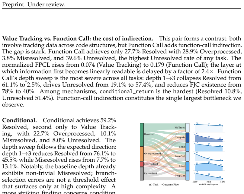
Function Call × depthexhibits the most extreme gradient in the entire dataset. Resolved rate collapses from 61.1% at depth=1 to a mere 2.5% at depth=3, while Unresolved surges from 19.1% to 57.4%. This near-total failure indicates that the model cannot reliably track values through deeply nested function calls—each additional call level compounds difficul...
-
[22]
The conditional_return mechanism yields only 10.8% Resolved and 51.4% Un- resolved, compared to 38.7% Resolved for arithmetic
Function Call × mechanismreveals sharp differentiation by function-body type. The conditional_return mechanism yields only 10.8% Resolved and 51.4% Un- resolved, compared to 38.7% Resolved for arithmetic. Conditional branching within function bodies severely undermines the model’s ability to complete the computation
-
[23]
Notably, the failure mode skews toward Overprocessed rather than Unresolved, indicating that the model caninitiatebut cannotsustainmulti-step arithmetic
Computing × stepsshows monotonic degradation: Resolved drops from 42.6% (2 steps) to 12.6% (4 steps), while Overprocessed climbs from 25.4% to 47.5%. Notably, the failure mode skews toward Overprocessed rather than Unresolved, indicating that the model caninitiatebut cannotsustainmulti-step arithmetic
-
[24]
Although unrolling removes loop syntax, computational complexity still overwhelms the model at higher repetition counts
Loop-unrolled × iterationsmirrors the Computing pattern: Resolved falls from 46.1% (2 iterations) to 11.8% (4 iterations), with Unresolved reaching 46.7% at the highest setting. Although unrolling removes loop syntax, computational complexity still overwhelms the model at higher repetition counts
-
[25]
55 Preprint
Value Tracking× distractorsdemonstrates that even the simplest task type pays a substantial cost for irrelevant context: Resolved drops from 86.6% (0 distractors) to 61.8% (2 distractors), while MR rises from 1.1% to 8.4%. 55 Preprint. Under review. H.3.2 Overprocessed Peaks The Overprocessed outcome—where the model once held the correct answer but subse-...
-
[26]
60 Preprint
Resolved% increases monotonically with scale(18.0% at 0.5B to 50.3% at 14B), indicating that larger models more reliably complete the full information lifecycle from availability to readiness. 60 Preprint. Under review
-
[27]
FPCLn decreases monotonically(0.214 to 0.120), meaning information becomes linearly decodable at proportionally earlier layers in larger models
-
[28]
The 14B model dips slightly to 0.343, possibly reflecting improved CSD capability that narrows the gap with probing
Normalized ∆brew exhibits a step-then-plateau pattern: 0.5B has a relatively narrow brewing interval (0.288), which widens sharply at 1.5B (0.390) and then stabilizes around 0.37–0.39 for 3B/7B. The 14B model dips slightly to 0.343, possibly reflecting improved CSD capability that narrows the gap with probing
-
[29]
Unresolved% drops substantially with scale(45.1% at 0.5B to 14.0% at 14B), while Overprocessed% remains relatively stable (22–34%), suggesting that scaling primar- ily converts Unresolved failures into successful Resolutions. 0.5B 1.5B 3B 7B 14B 0 20 40 60 80 100 Value Tracking 0.5B 1.5B 3B 7B 14B 0 20 40 60 80 100 Computing 0.5B 1.5B 3B 7B 14B 0 20 40 60...
-
[30]
Information consistently becomes linearly decodable before the model can autonomously decode it
The brewing-to-resolution structure is universal.All five models—spanning two architecture families—exhibit positive ∆brew on every task. Information consistently becomes linearly decodable before the model can autonomously decode it
-
[31]
The bottleneck lies in CSD capability (Figure 14)
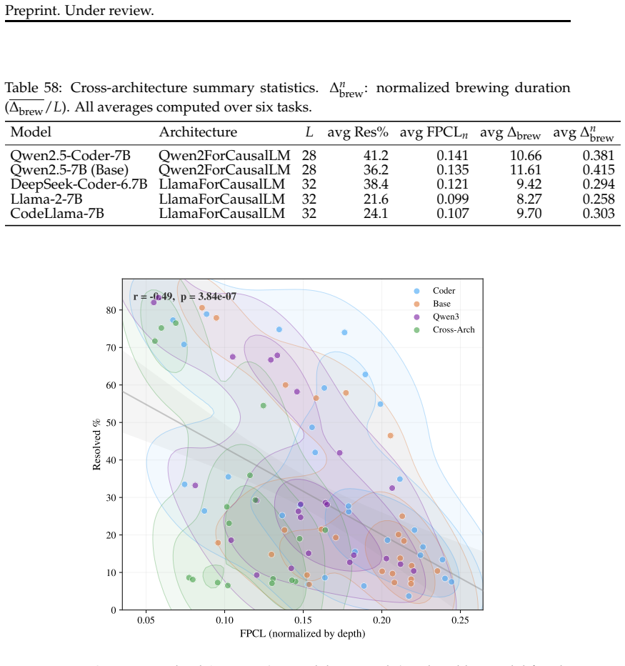
Resolved% varies widely across models, and the bottleneck is not information availability.Llama-2-7B has the lowest FPCL n among all models (0.099), mean- ing information becomes readable earliest, yet it achieves only 21.6% average Resolved%. The bottleneck lies in CSD capability (Figure 14)
-
[32]
Normalized ∆brew stratifies by architecture family.Qwen-family models exhibit wider brewing intervals (0.33–0.42), while Llama-family models show narrower intervals (0.26–0.30). Two possible explanations: (a) architectural differences lead to distinct information-availability-to-readiness transition dynamics, or (b) selection bias—in models with weaker CS...
-
[33]
Information reaches an available state but is subsequently degraded by later layers, reflecting insufficient integration of code reasoning capability in the residual stream
Llama-2 and CodeLlama exhibit dominant Overprocessed patterns.On computa- tionally intensive tasks (Computing, Loop, Loop-unrolled), Llama-2-7B’s Overpro- cessed rate ranges from 41.7% to 52.5%, far exceeding its Resolved rate (7.3–8.3%). Information reaches an available state but is subsequently degraded by later layers, reflecting insufficient integrati...
-
[34]
available but not delivered
DeepSeek-Coder-6.7B performs comparably to Qwen despite sharing the Llama architecture.Its average Resolved rate of 38.4% is on par with the Qwen models, confirming that the quality of code-specialized pre-training data is the dominant factor, not architectural choice. I.4 External-Benchmark Corroboration: CRUXEval-O CUE-Bench is a controlled, single-toke...
2024
discussion (0)
Sign in with ORCID, Apple, or X to comment. Anyone can read and Pith papers without signing in.