pith. sign in

arxiv: 2606.18332 · v1 · pith:JMLGRZKAnew · submitted 2026-06-16 · 🌌 astro-ph.IM · astro-ph.GA

The Via Project: Overview of the Science, Instrument, and Survey

Pith reviewed 2026-06-26 22:24 UTC · model grok-4.3

classification 🌌 astro-ph.IM astro-ph.GA
keywords spectroscopic surveyradial velocitystellar streamsdark matterMilky Way satellitescircumgalactic mediumtransient spectroscopyfiber spectrograph
0
0 comments X

The pith

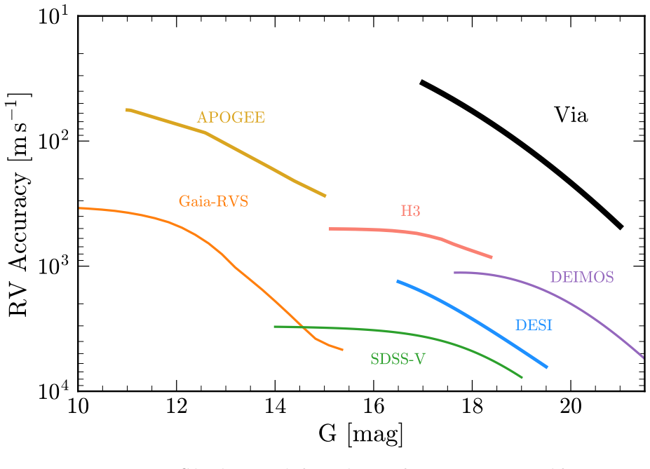
Via will achieve 100 m/s radial velocity stability for millions of faint stars while reaching single-visit depth for transient spectroscopy.

A machine-rendered reading of the paper's core claim, the machinery that carries it, and where it could break.

The paper outlines the Via Project as a planned five-year all-sky spectroscopic survey beginning in 2027 on two large telescopes. It deploys multi-object fiber systems to deliver precise radial velocities for over two million stars fainter than G=21 and spectra of transients down to r=24. Four primary goals focus on velocity perturbations in stellar streams, chemodynamics of satellite galaxies, absorption mapping of circumgalactic gas, and transient follow-up. These measurements are positioned to enable new probes in near-field cosmology and time-domain astrophysics.

Core claim

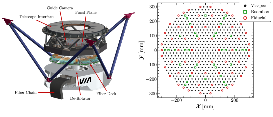
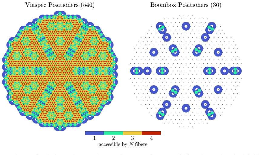
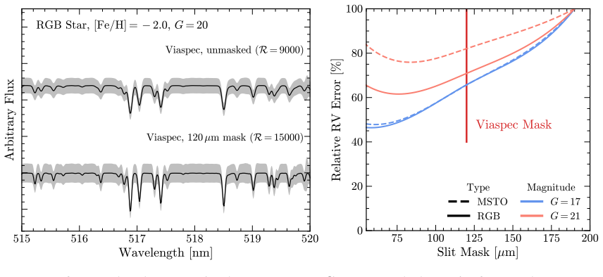
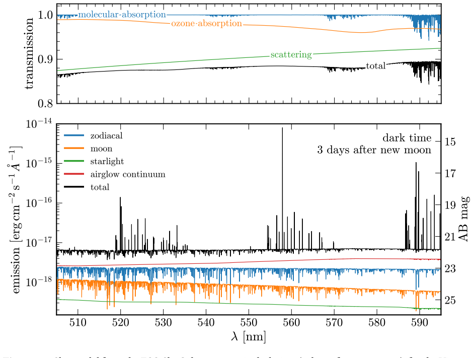
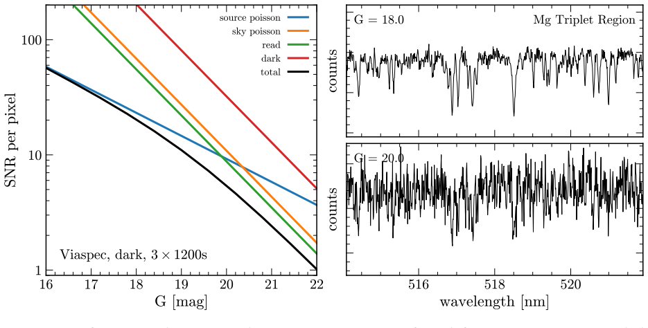
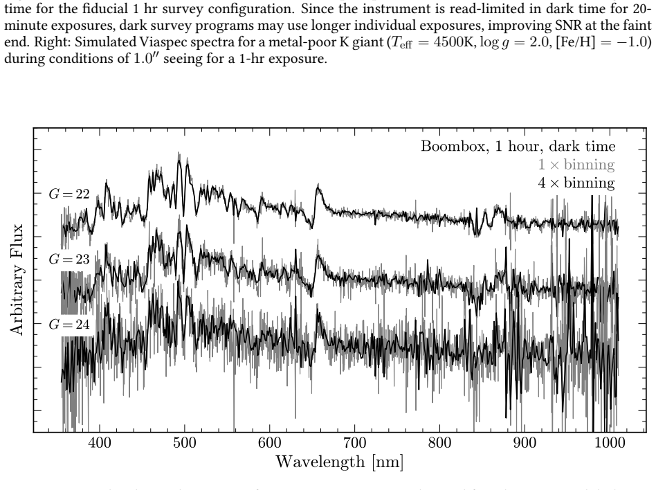
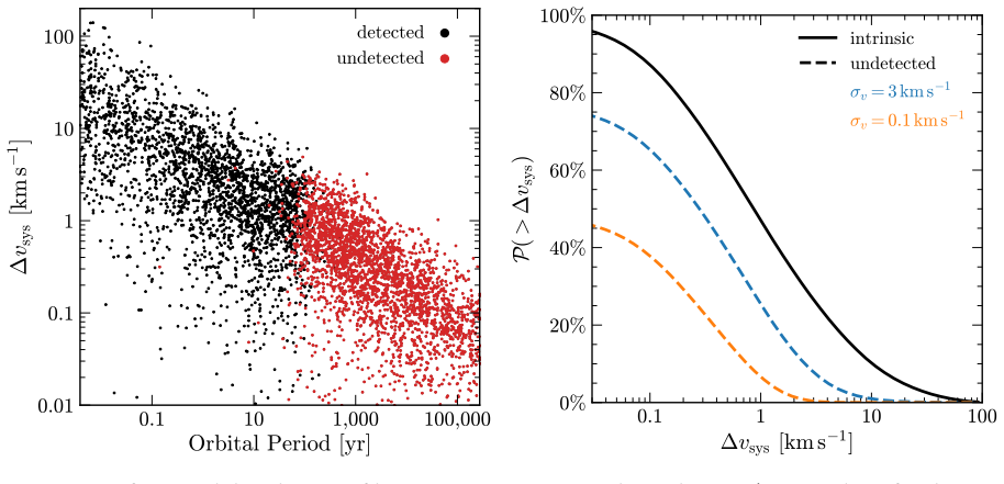
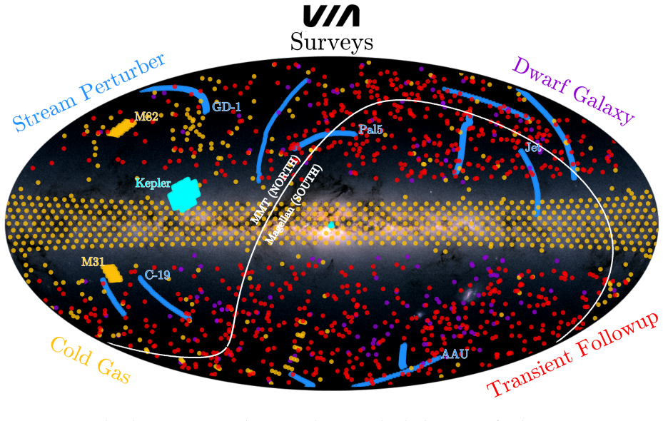
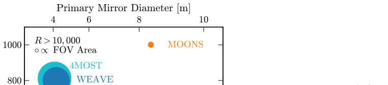
Via will deploy identical fiber-fed multi-object spectrographs on the MMT and Magellan/Clay telescopes for a five-year dual-hemisphere survey of more than two million stars, with each instrument using 576 robotically positioned fibers over a one-degree field to feed Viaspec at R approximately 15,000 and Boombox at R approximately 1,000, achieving 100 m/s radial velocity stability at G less than or equal to 21 and reaching r approximately 24 for transients.

What carries the argument

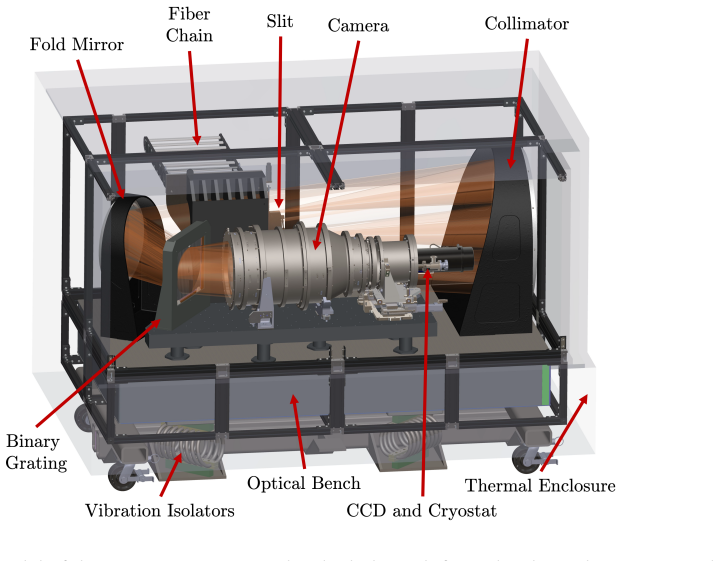
Robotically positioned fiber systems feeding the dual spectrographs Viaspec (high-resolution) and Boombox (low-resolution) over a one-degree field of view.

If this is right

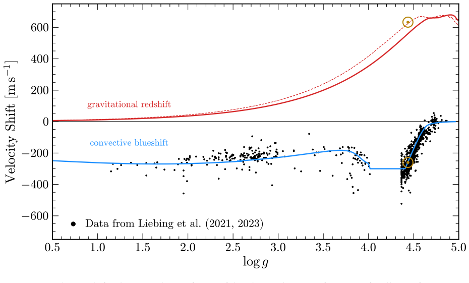
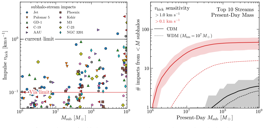
  • A comprehensive survey of velocity perturbations in cold stellar streams sensitive to subhalos with mass less than or equal to 10^7 solar masses, testing the particle nature of dark matter.
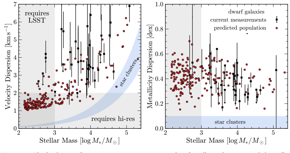
  • A chemodynamical census of Milky Way satellite galaxies to understand the formation of the faintest galaxies.
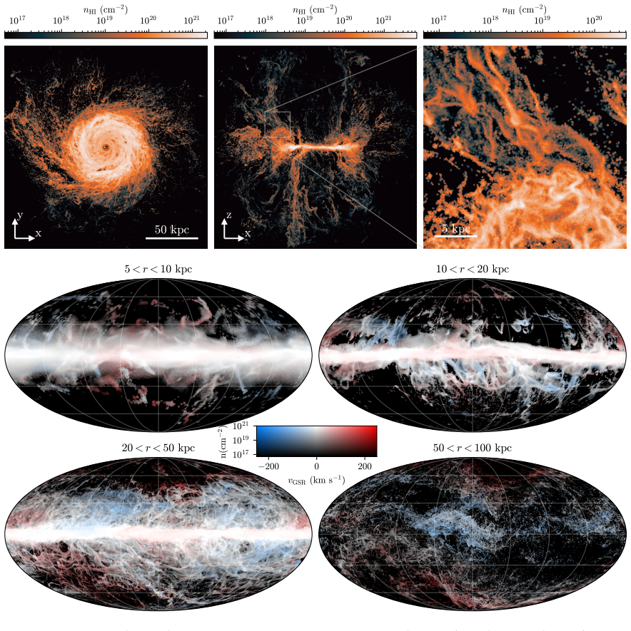
  • The first 3D tomographic maps of cold gas in the circumgalactic medium via NaI absorption.
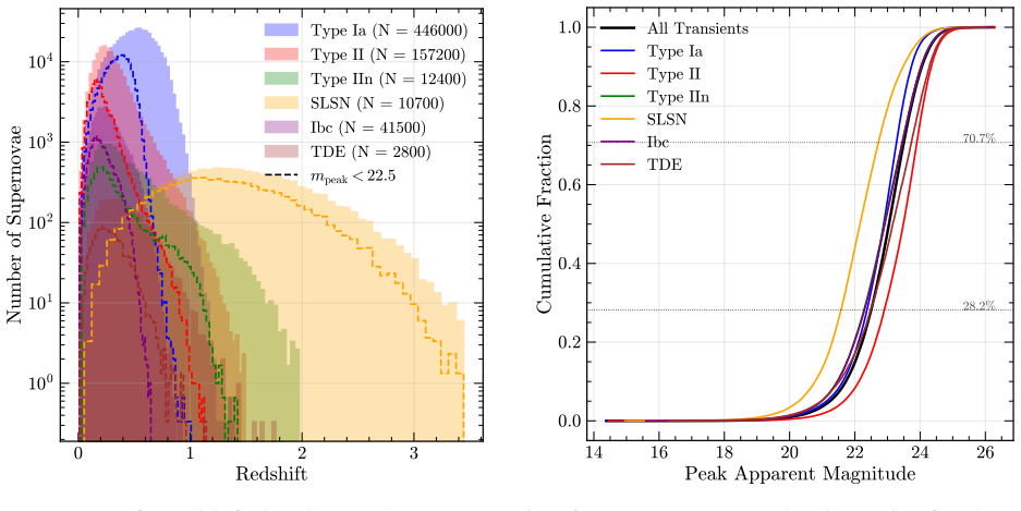
  • Rapid characterization of thousands of transients to the single-epoch survey depth.

Where Pith is reading between the lines

These are editorial extensions of the paper, not claims the author makes directly.

  • The subhalo detections would directly constrain the minimum mass scale of dark matter structure and thus the particle properties of dark matter.
  • Combined velocity and chemistry data could trace the accretion history of the Milky Way halo in greater detail than photometry alone.
  • Absorption-line maps would provide new constraints on the spatial distribution and kinematics of cold circumgalactic gas.
  • Spare-fiber observations could yield serendipitous results on polluted white dwarfs and high-redshift absorption systems.

Load-bearing premise

The robotically positioned fiber systems and dual spectrographs will be constructed, commissioned, and operated to deliver the stated performance metrics, and the five-year dual-hemisphere survey will receive the required telescope time allocations beginning in 2027.

What would settle it

Commissioning observations that fail to reach 100 m/s radial velocity stability on stars at G approximately 21, or the survey not receiving telescope time allocations to begin operations in 2027.

Figures

Figures reproduced from arXiv: 2606.18332 by The Via Collaboration.

Figure 1
Figure 1. Figure 1: A model of a 107 M⊙ dark matter subhalo flying through a stellar stream, at three points of time from left to right. The top panels show the 3D distribution of stars around the Milky Way, with stars colored by the impulsive velocity kick they receive from the passing subhalo. The central panels show the on-sky distribution of stars along the stream. The bottom panels show the radial velocity as a function … view at source ↗
Figure 2
Figure 2. Figure 2: The landscape of spectroscopic measurements in dwarf satellite galaxies around the Milky Way. As a function of stellar mass, the velocity dispersion (left) and metallicity dispersion (right) are shown for existing measurements (Pace 2025; Geha et al. 2026), and for a predicted population of LSST￾discoverable dwarf galaxies (Manwadkar & Kravtsov 2022). The locus of star clusters—whose kinematics and chemist… view at source ↗
Figure 3
Figure 3. Figure 3: Top: H i column density projections in Cartesian coordinates (Lucchini et al. 2026). Bottom: On-sky images of the H i column density colored by radial velocity. Each of the four panels shows the gas at a different distance range, viewed from a solar-like position 8 kpc from the Galactic center. phy of cold gas with low-dispersion spectrographs. The two strongest tracers of cold gas in the optical are Ca ii… view at source ↗
Figure 4
Figure 4. Figure 4: Left: Redshift distributions by transient class for a PLAsTiCC-simulated sample of realistic LSST transient light curves at a peak apparent-magnitude limit of mpeak = 23.5 (Kessler et al. 2019). Dashed curves show the reduced survey volume for a brighter limit of mpeak = 22.5, representative of 4MOST–TiDES. Right: Cumulative distribution of peak apparent magnitudes for the same transient classes. Percentil… view at source ↗
Figure 5
Figure 5. Figure 5: Overview of the Via instrument system, as shown deployed at the Magellan/Clay telescope. The fiber-positioning system (FPS) is secured to the back of the primary mirror at the focus of the f /5.3 secondary. The fiber run brings the optical fibers from the focal plane to the Viaspec and Boombox spec￾trographs, located on the azimuth disk. The metrology system resides in front of the secondary mirror. At the… view at source ↗
Figure 6
Figure 6. Figure 6: Left: CAD model of the Via fiber positioner in its full housing, with individual components labeled. Right: Layout of fiber positioners and fixed fiducials at the focal plane. The base positions of Viaspec (N = 540) and Boombox (N = 36) positioners are shown with circles and squares, respectively. Fixed fiducials (N = 60, open circles) will be used to set the physical coordinate system of the focal plane i… view at source ↗
Figure 7
Figure 7. Figure 7: The Via focal plane, showing the patrol regions of Viaspec (left) and Boombox (right) fiber positioners, colored by the number of positioners that can access a given region. The Viaspec patrol regions are highly overlapping, with ≳ 60% of the focal plane accessible by ≥ 3 Viaspec positioners. Boombox positioners are arranged in a pattern of linear spokes, so that arbitrary arrangements of high￾value transi… view at source ↗
Figure 8
Figure 8. Figure 8: Zemax lens drawing of the Viaspec optics. This drawing shows a top-down view of the spectro￾graph optical prescription. The fiber slit is defined perpendicular to the page. Only a single on-axis field point is drawn and the ray colors differentiate between wavelengths of light. cminutes off-axis. Each of the four units can move in an 80◦ segment of the annulus, accessing 44 sq. arcmin. of sky. The Shack–Ha… view at source ↗
Figure 9
Figure 9. Figure 9: CAD model of the Viaspec spectrograph. The light path from the slit to the camera is shown in orange. At the MMT, the fiber shoe need not be separated from the spectrograph when Viaspec is not in operation. An 800 mm diameter spherical mirror collimates the ≈ f/5.3 output light from each fiber into a 254 mm diameter pupil on the face of the grating. A fold mirror allows a more compact spectrograph layout. … view at source ↗
Figure 10
Figure 10. Figure 10: Throughput of different elements along the Viaspec optical path. The instrument throughput includes all components except the telescope, ADC (atmospheric dispersion compensator), and seeing￾dependent aperture losses. The total throughput includes telescope and ADC contributions. 500 520 540 560 580 600 Wavelength [nm] Arbitrary Flux [Fe/H] = -1.0 giant [Fe/H] = -1.0 MSTO [Fe/H] = -3.0 giant polluted white… view at source ↗
Figure 11
Figure 11. Figure 11: Example spectra demonstrating the Viaspec wavelength range and resolution, for a variety of core and ancillary science cases. The polluted white dwarf model is courtesy S. Blouin. The quasar is a Keck HIRES spectrum of B1422+2309 courtesy A. Cowie and the Keck Observatory Archive. 19 [PITH_FULL_IMAGE:figures/full_fig_p025_11.png] view at source ↗
Figure 12
Figure 12. Figure 12: Left: Simulated spectra (with 1σ errors at G = 20 in dark time) of a metal-poor RGB star observed with unmasked Viaspec fibers (top), and with a 120 µm slit placed at the fiber output. Right: Improvement in the derived RV uncertainty as a function of the width of the Viaspec slit mask, relative to the unmasked case. the unmasked case. For this test we assume a metal-poor [Fe/H]= −2.0 red giant branch star… view at source ↗
Figure 13
Figure 13. Figure 13: Left: Predicted throughput of the Boombox instrument, with and without the telescope con￾tribution. The sharp features arise from the expected throughput of the binary gratings. Right: Boombox fiber layout in the Via focal plane. The 36 fibers are arranged in a spoke design, allowing for pointing flex￾ibility. This sample field has 11 “active” transients (orange crosses) from a simulated LSST survey. With… view at source ↗
Figure 14
Figure 14. Figure 14: Number of objects that are assigned Boombox fibers, as a function of the total num￾ber of available Boombox targets. This is from a full simulation of the Boombox focal plane, in￾cluding “aiming” the center and rotation of the field. The black line (shaded band) indicates the mean (1σ distribution) from 1000 random real￾izations. The three highest-priority targets are guaranteed to be observed, and more t… view at source ↗
Figure 15
Figure 15. Figure 15: Zemax lens drawing of the Boombox optics. This drawing shows a top-down view of the spectrograph optical prescription. The fiber slit is defined perpendicular to the page. Only a single on-axis field point is drawn and the ray colors differentiate between wavelengths of light. 22 [PITH_FULL_IMAGE:figures/full_fig_p028_15.png] view at source ↗
Figure 16
Figure 16. Figure 16: The Boombox mechanical design. Light enters through the fiber slit (bottom right) and is collimated (bottom middle) before being split into red and blue channels by a dichroic. In both channels the light is dispersed by a grating and then re-imaged through a custom camera onto the detectors (light gray). The camera and collimator assemblies are made up of a stack of precision lens bezels for fine alignmen… view at source ↗
Figure 17
Figure 17. Figure 17: Example spectra demonstrating the Boombox wavelength range and science cases, including kilonovae, tidal disruption events, supernovae, and dwarf galaxies. The supernovae are examples from the PLAsTiCC database (Kessler et al. 2019). 2.5. The Fiber Run Via uses fiber optic cables to relay light from the focal plane to the spectrographs [PITH_FULL_IMAGE:figures/full_fig_p030_17.png] view at source ↗
Figure 18
Figure 18. Figure 18: Schematic layout of fiber optic cables connecting the focal plane system to Viaspec and Boom￾box. The fiducials are fixed position fibers used to measure the absolute positions of all fibers, and are fed to Viaspec, where they are also used as sky fibers during science observations. The calibration unit contains Pen-Ray lamps that are also fed to Viaspec. The number of fibers between each connection is sh… view at source ↗
Figure 19
Figure 19. Figure 19: A small portion of a simulated raw 2D Viaspec image from the data simulator. The image is zoomed in on 66 fibers near the Mg i triplet (located near the center of the image). Six calibration fibers are clearly visible as emission line spectra. 2.6. Data Simulator We have developed a full simulation of the telescope, Viaspec, and Boombox to realistically predict raw 2D detector images ( [PITH_FULL_IMAGE:f… view at source ↗
Figure 20
Figure 20. Figure 20: Sky model from the ESO SkyCalc program, in dark time (3 days after new moon), for the Viaspec wavelength range and resolution. The top panel shows the sky transmission from molecular absorption lines (telluric features). Including all absorption and scattering components, the total sky transmission in the Viaspec wavelength range is ≈ 88% at zenith. The bottom panel shows the various sky emission componen… view at source ↗
Figure 21
Figure 21. Figure 21: Left: Fractional noise contribution to Viaspec spectra from different sources, assuming dark time for the fiducial 1 hr survey configuration. Since the instrument is read-limited in dark time for 20- minute exposures, dark survey programs may use longer individual exposures, improving SNR at the faint end. Right: Simulated Viaspec spectra for a metal-poor K giant (Teff = 4500K, log g = 2.0, [Fe/H] = −1.0)… view at source ↗
Figure 22
Figure 22. Figure 22: Simulated Boombox spectra for a Type IIP supernova observed for 1 hr in nominal dark con￾ditions. The G magnitude of each spectrum is indicated, and spectra are shown with 1× and 4× spectral binning. 28 [PITH_FULL_IMAGE:figures/full_fig_p034_22.png] view at source ↗
Figure 23
Figure 23. Figure 23: Left: Median Viaspec SNR versus G magnitude for a variety of seeing conditions in dark time (0% lunar illumination), at the survey depth of 1 hr and the deep-drilling depth of 10 hr. Right: Analogous SNR curves for Boombox with 1-hr exposures, shown for dark and bright time. is 18 e − hr−1 per pixel. Boombox’s much lower resolution means that these are not dominant terms in the error budget. The left pane… view at source ↗
Figure 24
Figure 24. Figure 24: Predicted radial velocity (left), [Fe/H] (center), and [α/Fe] (right) precision for mock red giant branch (RGB) and main-sequence turn-off (MSTO) stars, as a function of the SNR per pixel. The top axis shows corresponding Gaia G magnitudes for 1 effective hour of observations. The metallicity used when generating each mock is indicated by the line colors provided in the legend. Errors are shown with and w… view at source ↗
Figure 25
Figure 25. Figure 25: Radial velocity jitter as a function of surface gravity for giants observed with the TRES spec￾trograph (D. Latham, priv. comm), giants from Spaeth et al. (2025), and dwarfs observed with Keck/HIRES (Luhn et al. 2020, 2023). The TRES sample includes bright giants from the Hipparcos survey, and metal￾poor giants associated with the Gaia–Sausage–Enceladus (GSE) merger. Binary orbital solutions have been fit… view at source ↗
Figure 26
Figure 26. Figure 26: Left: Period distribution of binaries in our numerical simulation. ∆vsys is the offset between the mean RV measured by the survey (if we assumed all epoch measurements come from a single star), and the intrinsic center-of-mass velocity of the binary. Note that this is different from the binary semi￾amplitude K, which is the worst-case value of ∆vsys for a given system. Right: The probability that a binary… view at source ↗
Figure 27
Figure 27. Figure 27: Velocity shift relative to the restframe of the photosphere as a function of stellar surface gravity. The gravitational redshift effect is shown along an isochrone for [Fe/H]= 0 at 5 Gyr (dashed red line) and [Fe/H]= −2 at 10 Gyr (solid red line). Convective blueshifts measured by Liebing et al. (2021, 2023) are shown as open symbols. A simple model for convective blueshifts is shown as a blue line, in wh… view at source ↗
Figure 28
Figure 28. Figure 28: Idealized simulation of a stream after directly encountering a 107 M⊙ subhalo, showing the radial velocity perturbation as a function of longitude along the stream. The stream is sampled as a 104M⊙ stellar population at a distance of 20 kpc (analogous to the Pal-5 stream), and magnitude-dependent ob￾servational uncertainties are added for two survey configurations. The red line fits the characteristic 1/ϕ… view at source ↗
Figure 29
Figure 29. Figure 29: Left: Simulation of subhalo–stream impacts showing the impulsive kick velocity vkick as a function of subhalo mass at the time of the impact. The subhalos are drawn from a semi-analytic sim￾ulation of a Milky Way-like galaxy assuming cold dark matter (CDM), and the streams are simulated to match real streams in the Milky Way (Chandra et al, in prep). Radial velocity stability limits for current surveys (1… view at source ↗
Figure 30
Figure 30. Figure 30: Left: Number of targets in dwarf galaxies of varying mass and distance, for a G < 23 limiting magnitude corresponding to 10 hr Viaspec depth. We assume a [Fe/H] = −2.0, 12 Gyr stellar population and a Kroupa IMF for this test. Right: Fraction of dwarf galaxy stars observable by the Via fiber positioner in a single pointing, as a function of the number of visible stars and the apparent half-light radius. T… view at source ↗
Figure 31
Figure 31. Figure 31: Simulating Via observations of the most dark matter dominated galaxy known, Segue 1. Left: Spatial distribution of Segue 1 members, observed with a realistic simulation of the Via fiber positioner. The 1-degree FoV of the fiber positioner is shown in red, and ellipses denote 2, 4, and 6 half-light radii of Segue 1. A single pointing can observe 43 members (red points), and 5 pointings (fiber configuration… view at source ↗
Figure 32
Figure 32. Figure 32: Forecast for the Via survey of dwarf galaxies discovered by LSST, showing stellar mass as a function of half-light radius (left) and heliocentric distance (right). Open markers show currently known dwarfs with measured velocity dispersions (Pace 2025), and colored markers show predicted dwarfs that LSST will discover, and for which Via will deliver > 5 stellar spectra in a single pointing. LSST prediction… view at source ↗
Figure 33
Figure 33. Figure 33: Simulated spectrum of an RGB star acting as a backlight for gas along the line of sight at a relative velocity of −50 km s−1 , observed at R = 3000 (blue) and R = 15000 (red). At the resolution of Viaspec, Na i absorption from cold gas can be disentangled from stellar absorption, revealing the density and velocity structure of the interstellar and circumgalactic medium. Substantially higher spectral resol… view at source ↗
Figure 34
Figure 34. Figure 34: Relation between Na i 589.0/589.6nm EW (in Å) and spec￾trum SNR per pixel for a Na i detec￾tion threshold of 3σ. Na i EW is con￾verted to an approximate H i column density along the right axis (Murga et al. 2015). Limiting G-band magni￾tude at a given SNR is shown along the top axis. Sensitivity to cold gas will be determined by both the signal-to-noise ratio of individual spectra and the number of stars … view at source ↗
Figure 35
Figure 35. Figure 35: Distribution of stellar sources along two example sight-lines, according to the GUMS mock catalog (Robin et al. 2012). The Galactic plane sightline intersects Complex H, for which the only direct distance measurement for the gas is a 6 kpc lower limit (Smoker et al. 2011). The high-latitude sightline intersects Complex C, which is currently bracketed at 10 ± 2.5 kpc. We also expect multiple quasars per fi… view at source ↗
Figure 36
Figure 36. Figure 36: Scales probed by stars behind a no￾tional gas cloud at (l, b) = (198◦ , 35◦ ) and a distance of 200 pc. Small-scale structure can be detected by measuring a pair of nearby stars simultaneously, or by measuring a single star with a high proper motion over the 5-year sur￾vey baseline [PITH_FULL_IMAGE:figures/full_fig_p056_36.png] view at source ↗
Figure 37
Figure 37. Figure 37: Four major target categories for the Boombox time-domain program. Each colored box rep￾resents the typical luminosity and redshift range of a target class: gravitational-wave counterparts and kilonovae (GW / KNe), young core-collapse supernovae and precursor events (Young SNe / Precursors), rare or anomalous transients (Anomalous), and passively selected active supernovae in Via fields (Passive SNe). The … view at source ↗
Figure 38
Figure 38. Figure 38: The Lyman-alpha forest of the z = 3.62 quasar B1422+2309, which covers half the Viaspec wavelength range. The top spectrum is an observation by the R ≈ 48,000 Keck/HIRES instrument (top; Songaila & Cowie 1996). The middle spectrum is smoothed to the Viaspec resolution, and the bottom spectrum is “observed” for 1 hour in dark time with the full Viaspec data simulator. surement of the patchiness of He ii bu… view at source ↗
Figure 39
Figure 39. Figure 39: Left: Simulated Lyman-alpha forest spectra at z = 3.1 for two different IGM temperature parameters T0, as observed by a low-resolution survey like DESI (top) and at Viaspec resolution (bottom). Right: Results from fitting a mock Via survey of 1000 quasars drawn from the Quaia quasar catalog. This mock survey recovers the evolution of the IGM’s thermal state from z = 3–4, in this case recovering the temper… view at source ↗
Figure 40
Figure 40. Figure 40: The impact of 1000 fast radio burst host galaxies measured by Boombox. Black points on the left figure shows a simulated distribution of extragalactic dispersion measures vs. redshift for FRB host galaxies measured by Boombox, with 20 < r < 24 and 0 < z < 1.3. The bottom panel shows the corresponding constraints on the IGM and its redshift evolution. The right figure shows constraints on the baryon power … view at source ↗
Figure 41
Figure 41. Figure 41 [PITH_FULL_IMAGE:figures/full_fig_p066_41.png] view at source ↗
Figure 42
Figure 42. Figure 42: Simulated spectrum tuned to match Comet C/2014 Q2, generated with the NASA-GSFC Plan￾etary Spectrum Generator (Villanueva et al. 2018). Emission lines from three different carbon-bearing molecules are highlighted. puts Via squarely in the regime needed for eclipsing and astrometric binary rejection. The var￾ious exoplanet samples will benefit from Via’s sky coverage. Gaia will have an enhanced yield in th… view at source ↗
Figure 43
Figure 43. Figure 43: Simulated Via program to observe the Kepler field. The entire field can be observed in 189 separate Via pointings (left panel), enabling uniform spectroscopic coverage over ≈ 100 sq. deg. The right panel shows the number of stars observed as a function of G-band magnitude and SNR. The latter was estimated from the Via ETC assuming 5m exposures in bright moon conditions. Assuming 5m overheads, a single pas… view at source ↗
Figure 44
Figure 44. Figure 44: Simulated Via Survey in Galactic coordinates. Individual pointings for the Via primary surveys are shown as colored circles (not to scale) and are overlaid on an all-sky image of the Galaxy. Several individual targets are labeled. The white line indicates the equatorial plane. This is a single realization of one possible survey configuration. 4.2.2. Dedicated Pointings A Complete Census of the Kepler Fiel… view at source ↗
Figure 45
Figure 45. Figure 45: Cumulative distribution of the number of times a target will be observed by Via (Nvisit) under the nominal survey strategy. Approximately 104 objects will be visited at least 10 times. The separa￾tion between successive observations will range from days to years. CGS = cold gas survey, DGS = dwarf galaxy survey, SPS = stream perturbation survey, and TFS = transient followup survey. added in special circum… view at source ↗
Figure 46
Figure 46. Figure 46: Schematic showing the Compass pipeline for modeling realizations of the Milky Way and its accreted stellar substructure. Teal boxes indicate simulation data products; red text indicates tools and tunable models that produce them. The yellow box indicates the readily repeatable modeling steps that can generate realizations over parameter spaces. Examples of comparisons of specific mock observables to data … view at source ↗
Figure 47
Figure 47. Figure 47: Left: The observed radial velocity structure of a stream (top, “Data”) compared against nu￾merous forward-modeled realizations (bottom, “Sims”) under a specified dark matter model. The models rapidly capture the stochastic perturbations in radial velocity (∆vr) along the stream coordinate (ϕ1) in￾duced by subhalo impacts. Center: A suite of summary statistics computed for both the observed data and the si… view at source ↗
Figure 48
Figure 48. Figure 48: Performance of Viaspec and the most comparable wide-field spectrograph on a 6m-class telescope, MMT/Hectochelle. Points show observed data from the H3 Survey (Conroy et al. 2019), which were observed in bright time with 30 min exposures. Blue curves show predictions from the Data Simulator (§2.6) configured with Hectochelle parameters; the two seeing values bracket typical conditions at the MMT. The red c… view at source ↗
Figure 49
Figure 49. Figure 49: Current and forthcoming multi-object spectroscopic instruments with R > 10, 000, compared to Viaspec along two axes: the primary mirror collecting area, and number of fibers in a single pointing. Marker sizes are proportional to the FoV area. FoV and 360–980 nm coverage at R ∼ 2000–5000. DESI’s relatively low resolution precludes the high velocity precision required here. (2) The SDSS-V, operating at 2.5m… view at source ↗
Figure 50
Figure 50. Figure 50: RV accuracy vs. G-band magnitude for a selection of previous, ongoing, and future surveys. Here “accuracy” is defined as the quadrature sum of the magnitude-dependent RV precision, and the sys￾tematic RV stability floor of the instrument (typically determined via repeat observations). The predicted Via precision for a [Fe/H]= −1 RGB star is shown. For comparison, we show APOGEE (Price-Whelan et al. 2020; … view at source ↗
read the original abstract

Via is a forthcoming all-sky spectroscopic survey that will achieve 100 m s$^{-1}$ radial velocity stability for millions of faint ($G \lesssim 21$) stars while reaching LSST's single-visit depth ($r \approx 24$) for transient spectroscopy, opening new regimes in near-field cosmology and time-domain astrophysics. Via will deploy identical fiber-fed, multi-object spectrographs on the 6.5m MMT and Magellan/Clay telescopes for a five-year, dual-hemisphere survey of $>2{,}000{,}000$ stars beginning in 2027 - timed to complement LSST. Each instrument has 576 robotically positioned fibers over a $1^\circ$ field of view, feeding two spectrographs: Viaspec ($R \approx 15{,}000$; 505-595 nm; 540 fibers) and Boombox ($R \approx 1{,}000$; 360-1010 nm; 36 fibers). Four key goals drive the survey: (1) a comprehensive survey of velocity perturbations in cold stellar streams, sensitive to $M \lesssim 10^7$ subhalos below the threshold of galaxy formation, a stringent test of the particle nature of dark matter; (2) a chemodynamical census of Milky Way satellite galaxies to understand the formation of the faintest galaxies; (3) the first 3D tomographic maps of cold gas in the circumgalactic medium via NaI absorption; and (4) the rapid characterization of thousands of transients to the single-epoch survey depth of LSST. Ancillary science - including the Ly$\alpha$ forest at $z \approx 3$-$4$, polluted white dwarfs, exoplanet host characterization, fast radio burst host galaxies, and extragalactic dwarf galaxies - will leverage spare fibers in every pointing. The Via Project is a collaboration between the Center for Astrophysics $|$ Harvard & Smithsonian, Carnegie Observatories, Stanford University, and Yale University.

Editorial analysis

A structured set of objections, weighed in public.

Desk editor's note, referee report, simulated authors' rebuttal, and a circularity audit. Tearing a paper down is the easy half of reading it; the pith above is the substance, this is the friction.

Referee Report

0 major / 1 minor

Summary. The manuscript is an overview of the Via Project, a planned dual-hemisphere spectroscopic survey deploying identical 576-fiber instruments on the MMT and Magellan/Clay 6.5 m telescopes beginning in 2027. It describes four primary science goals (velocity perturbations in cold stellar streams for subhalo detection, chemodynamical census of Milky Way satellites, 3D Na I tomography of the CGM, and rapid transient spectroscopy to LSST single-visit depth), the instrument architecture (Viaspec at R≈15,000 with 540 fibers and Boombox at R≈1,000 with 36 fibers), target performance (100 m s^{-1} RV stability for G≲21 stars), and ancillary programs leveraging spare fibers.

Significance. If the stated design targets are realized, the survey would open new parameter space in near-field cosmology by probing dark-matter subhalos below 10^7 M_⊙ and in time-domain astrophysics by matching LSST depth for transients. The dual-hemisphere strategy, robotic fiber positioning over 1° fields, and explicit complementarity with LSST constitute clear strengths of the concept. As a project-overview paper rather than a results paper, its primary value is to document the science case, instrument specifications, and survey timeline for the community.

minor comments (1)
  1. The abstract and §1 state the 100 m s^{-1} RV stability target without reference to an error budget or prototype data; while appropriate for an overview, a brief forward reference to where such supporting material will appear (if planned) would improve clarity for readers.

Simulated Author's Rebuttal

0 responses · 0 unresolved

We thank the referee for their positive assessment of the manuscript and recommendation to accept. The referee's summary correctly identifies the core elements of the Via Project overview, including the dual-hemisphere survey design, instrument specifications, science goals, and complementarity with LSST.

Circularity Check

0 steps flagged

No significant circularity; descriptive project overview only

full rationale

The paper is a high-level description of planned instrumentation, survey strategy, and science goals for the Via Project. It states design targets (e.g., 100 m s^{-1} RV stability, fiber counts, resolving powers, survey depth) and anticipated reach as engineering and allocation objectives, with no derivations, equations, fitted parameters, or predictions that reduce to input quantities by construction. No load-bearing self-citations, uniqueness theorems, or ansatzes are invoked. The document is self-contained as a project prospectus against external benchmarks of telescope time and instrument performance.

Axiom & Free-Parameter Ledger

0 free parameters · 0 axioms · 0 invented entities

No free parameters, axioms, or invented entities are introduced because the document is a descriptive project overview without theoretical derivations or data fitting.

pith-pipeline@v0.9.1-grok · 5898 in / 1453 out tokens · 36653 ms · 2026-06-26T22:24:17.915434+00:00 · methodology

discussion (0)

Sign in with ORCID, Apple, or X to comment. Anyone can read and Pith papers without signing in.

Reference graph

Works this paper leans on

300 extracted references · 299 canonical work pages · 14 internal anchors

  1. [1]

    P., Abbott, R., Abbott, T

    Abbott, B. P., Abbott, R., Abbott, T. D., et al. 2017, PhRvL, 119, 161101, doi: 10.1103/PhysRevLett.119.161101

  2. [2]

    K., Parikh, A., Slone, O., et al

    Adams, D. K., Parikh, A., Slone, O., et al. 2025, ApJ, 991, 66, doi: 10.3847/1538-4357/adf740

  3. [3]

    I., et al

    Agertz, O., Pontzen, A., Read, J. I., et al. 2020, MNRAS, 491, 1656, doi: 10.1093/mnras/stz3053

  4. [4]

    2024, The Astrophysical Journal, 974, 172, doi: 10.3847/1538-4357/ad6869 Allende Prieto, C., Koesterke, L., Ludwig, H

    Aleo, P., Engel, A., Narayan, G., et al. 2024, The Astrophysical Journal, 974, 172, doi: 10.3847/1538-4357/ad6869 Allende Prieto, C., Koesterke, L., Ludwig, H. G.,

  5. [5]

    2013, A&A, 550, A103, doi: 10.1051/0004-6361/201220064

    Freytag, B., & Caffau, E. 2013, A&A, 550, A103, doi: 10.1051/0004-6361/201220064

  6. [6]

    White, S. D. M. 2016, MNRAS, 463, L17, doi: 10.1093/mnrasl/slw148

  7. [7]

    P., Rey, M

    Andersson, E. P., Rey, M. P., Pontzen, A., et al. 2025, ApJ, 978, 129, doi: 10.3847/1538-4357/ad99d6

  8. [8]

    Robust Data-driven Metallicities for 175 Million Stars from Gaia XP Spectra

    Andrae, R., Rix, H.-W., & Chandra, V. 2023, ApJS, 267, 8, doi: 10.3847/1538-4365/acd53e

  9. [9]

    S., et al

    Andreoni, I., Margutti, R., Salafia, O. S., et al. 2022, ApJS, 260, 18, doi: 10.3847/1538-4365/ac617c

  10. [10]

    W., Perley, D

    Andreoni, I., Coughlin, M. W., Perley, D. A., et al. 2022, Nature, 612, 430, doi: 10.1038/s41586-022-05465-8

  11. [11]

    2024, arXiv e-prints, arXiv:2411.04793, doi: 10.48550/arXiv.2411.04793

    Andreoni, I., Margutti, R., Banovetz, J., et al. 2024, arXiv preprint arXiv:2411.04793, doi: 10.48550/arXiv.2411.04793

  12. [12]

    2018, ApJL, 855, L23, doi: 10.3847/2041-8213/aab267

    Arcavi, I. 2018, ApJL, 855, L23, doi: 10.3847/2041-8213/aab267

  13. [13]

    E., et al

    Arora, A., Garavito-Camargo, N., Sanderson, R. E., et al. 2024, ApJ, 974, 286, doi: 10.3847/1538-4357/ad7375

  14. [14]

    S., et al

    Augustin, R., Tumlinson, J., Peeples, M. S., et al. 2025, FOGGIE X: Characterizing the Small-Scale Structure of the CGM and its Imprint on Observables, doi: 10.3847/1538-4357/ae0462

  15. [15]

    2024, A&A, 683, A14, doi: 10.1051/0004-6361/202347848

    Awad, P., Canducci, M., Balbinot, E., et al. 2024, A&A, 683, A14, doi: 10.1051/0004-6361/202347848

  16. [16]

    2019, MNRAS, 484, 2009, doi: 10.1093/mnras/stz142

    Banik, N., & Bovy, J. 2019, MNRAS, 484, 2009, doi: 10.1093/mnras/stz142

  17. [17]

    Boer, T. J. L. 2021, MNRAS, 502, 2364, doi: 10.1093/mnras/stab210

  18. [18]

    2023, MNRAS, 523, 428, doi: 10.1093/mnras/stad1395

    Barry, M., Wetzel, A., Chapman, S., et al. 2023, MNRAS, 523, 428, doi: 10.1093/mnras/stad1395

  19. [19]

    The Discovery and Analysis of Very Metal-Poor Stars in the Galaxy

    Beers, T. C., & Christlieb, N. 2005, ARA&A, 43, 531, doi: 10.1146/annurev.astro.42.053102.134057

  20. [20]

    2022, MNRAS, 514, 689, doi: 10.1093/mnras/stac1267

    Belokurov, V., & Kravtsov, A. 2022, MNRAS, 514, 689, doi: 10.1093/mnras/stac1267

  21. [21]

    Benson, A. J. 2012, NewA, 17, 175, doi: 10.1016/j.newast.2011.07.004

  22. [22]

    2018, RvMP, 90, 045002, doi: 10.1103/RevModPhys.90.045002

    Bertone, G., & Hooper, D. 2018, RvMP, 90, 045002, doi: 10.1103/RevModPhys.90.045002

  23. [23]

    doi:10.1016/j.physrep.2004.08.031 , eprint =

    Bertone, G., Hooper, D., & Silk, J. 2005, PhR, 405, 279, doi: 10.1016/j.physrep.2004.08.031

  24. [24]

    and Xue, Xiang-Xiang and Liu, Chao and Shen, Juntai and Flynn, Chris and Yang, Chengqun and Zhao, Gang and Tian, Hai-Jun , title="

    Bird, S. A., Xue, X.-X., Liu, C., et al. 2021, ApJ, 919, 66, doi: 10.3847/1538-4357/abfa9e —. 2022, MNRAS, 516, 731, doi: 10.1093/mnras/stac2036

  25. [25]

    P., & Turok, N

    Bode, P., Ostriker, J. P., & Turok, N. 2001, ApJ, 556, 93, doi: 10.1086/321541

  26. [26]

    M., Wang, J., Zinn, J

    Boley, K. M., Wang, J., Zinn, J. C., et al. 2021, AJ, 162, 85, doi: 10.3847/1538-3881/ac0e2d

  27. [27]

    S., & Schlegel, D

    Bolton, A. S., & Schlegel, D. J. 2010, PASP, 122, 248, doi: 10.1086/651008

  28. [28]

    Hogg, D. W. 2019a, ApJL, 881, L37, doi: 10.3847/2041-8213/ab36ba

  29. [29]

    Bonaca, D

    Conroy, C. 2019b, ApJ, 880, 38, doi: 10.3847/1538-4357/ab2873

  30. [30]

    Bonaca, A., & Price-Whelan, A. M. 2025, NewAR, 100, 101713, doi: 10.1016/j.newar.2024.101713

  31. [31]

    M., et al

    Bonaca, A., Pearson, S., Price-Whelan, A. M., et al. 2020a, ApJ, 889, 70, doi: 10.3847/1538-4357/ab5afe

  32. [32]

    W., et al

    Bonaca, A., Conroy, C., Hogg, D. W., et al. 2020b, ApJL, 892, L37, doi: 10.3847/2041-8213/ab800c

  33. [33]

    2020, MNRAS, 495, 1374, doi: 10.1093/mnras/staa1246

    Bonnerot, C., & Lu, W. 2020, MNRAS, 495, 1374, doi: 10.1093/mnras/staa1246

  34. [34]

    A., Frenk, C

    Bose, S., Hellwing, W. A., Frenk, C. S., et al. 2016, MNRAS, 455, 318, doi: 10.1093/mnras/stv2294

  35. [35]

    2013, ApJ, 768, 70, doi: 10.1088/0004-637X/768/1/70

    Bovy, J., & Dvorkin, C. 2013, ApJ, 768, 70, doi: 10.1088/0004-637X/768/1/70

  36. [36]

    2020, ApJ, 898, 71, doi: 10.3847/1538-4357/ab9d85

    Breivik, K., Coughlin, S., Zevin, M., et al. 2020, ApJ, 898, 71, doi: 10.3847/1538-4357/ab9d85 —. 2021, COSMIC: Compact Object Synthesis and Monte Carlo Investigation Code. http://ascl.net/2108.022 84

  37. [37]

    2020, ApJ, 890, 73, doi: 10.3847/1538-4357/ab6989

    Bricman, K., & Gomboc, A. 2020, ApJ, 890, 73, doi: 10.3847/1538-4357/ab6989

  38. [38]

    2025, A&A, 703, A61, doi: 10.1051/0004-6361/202554642

    Podsiadlowski, P. 2025, A&A, 703, A61, doi: 10.1051/0004-6361/202554642

  39. [39]

    J., Gal-Yam, A., Yaron, O., et al

    Bruch, R. J., Gal-Yam, A., Yaron, O., et al. 2023, ApJ, 952, 119, doi: 10.3847/1538-4357/acd8be

  40. [40]

    O., Wechsler, R

    Buch, D., Nadler, E. O., Wechsler, R. H., & Mao, Y.-Y. 2024, ApJ, 971, 79, doi: 10.3847/1538-4357/ad554c

  41. [41]

    S., & Johnston, K

    Bullock, J. S., & Johnston, K. V. 2005, ApJ, 635, 931, doi: 10.1086/497422

  42. [42]

    S., Kravtsov, A

    Bullock, J. S., Kravtsov, A. V., & Weinberg, D. H. 2000, ApJ, 539, 517, doi: 10.1086/309279

  43. [43]

    2022, AJ, 164, 94, doi: 10.3847/1538-3881/ac76cc

    Bundy, K., Law, D., MacDonald, N., et al. 2022, AJ, 164, 94, doi: 10.3847/1538-3881/ac76cc

  44. [44]

    R., & Werk, J

    Quinn, T. R., & Werk, J. K. 2024, MNRAS, 535, 1672, doi: 10.1093/mnras/stae2459

  45. [45]

    S., Nakum, S., Ponnada, S

    Butsky, I. S., Nakum, S., Ponnada, S. B., et al. 2023, MNRAS, 521, 2477, doi: 10.1093/mnras/stad671

  46. [46]

    B., Koposov, S

    Buttry, R., Pace, A. B., Koposov, S. E., et al. 2022, MNRAS, 514, 1706, doi: 10.1093/mnras/stac1441 Byström, A., Koposov, S. E., Lilleengen, S., et al. 2025, MNRAS, 542, 560, doi: 10.1093/mnras/staf1219

  47. [47]

    2023, MNRAS, 525, 3499, doi: 10.1093/mnras/stad2512

    Font-Ribera, A., & Pedersen, C. 2023, MNRAS, 525, 3499, doi: 10.1093/mnras/stad2512

  48. [48]

    , archivePrefix = "arXiv", eprint =

    Cappellari, M. 2017, MNRAS, 466, 798, doi: 10.1093/mnras/stw3020

  49. [49]

    and Conroy, Charlie and Johnson, Benjamin D

    Cargile, P. A., Conroy, C., Johnson, B. D., et al. 2020, ApJ, 900, 28, doi: 10.3847/1538-4357/aba43b

  50. [50]

    Carlberg, R. G. 2009, ApJL, 705, L223, doi: 10.1088/0004-637X/705/2/L223 —. 2012, ApJ, 748, 20, doi: 10.1088/0004-637X/748/1/20 —. 2020, ApJ, 889, 107, doi: 10.3847/1538-4357/ab61f0

  51. [51]

    B., & Morse, J

    Laird, J. B., & Morse, J. A. 2003, AJ, 125, 293, doi: 10.1086/345386

  52. [52]

    2011, A&A, 530, A138, doi: 10.1051/0004-6361/201016276

    Casagrande, L., Schönrich, R., Asplund, M., et al. 2011, A&A, 530, A138, doi: 10.1051/0004-6361/201016276

  53. [53]

    S., Pace, A

    Cerny, W., Li, T. S., Pace, A. B., et al. 2026, arXiv e-prints, arXiv:2602.17652, doi: 10.48550/arXiv.2602.17652

  54. [54]

    B., & Mahabal, A

    Chaini, S., Bianco, F. B., & Mahabal, A. 2025, arXiv preprint arXiv:2510.23702, doi: 10.48550/arXiv.2510.23702

  55. [55]

    D., Craig, P

    Chakrabarti, S., Simon, J. D., Craig, P. A., et al. 2023, AJ, 166, 6, doi: 10.3847/1538-3881/accf21

  56. [56]

    O., Bernardinelli, P

    Chandler, C. O., Bernardinelli, P. H., Jurić, M., et al. 2026, The Astrophysical Journal, 1001, L35, doi: 10.3847/2041-8213/ae4b3a

  57. [57]

    and Conroy, Charlie and Ji, Alexander P

    Chandra, V., Naidu, R. P., Conroy, C., et al. 2023, ApJ, 951, 26, doi: 10.3847/1538-4357/accf13

  58. [58]

    2022, MNRAS, 513, 934, doi: 10.1093/mnras/stac933

    Chen, L.-H., Magg, M., Hartwig, T., et al. 2022, MNRAS, 513, 934, doi: 10.1093/mnras/stac933

  59. [59]

    Chevalier, R. A. 2012, ApJL, 752, L2, doi: 10.1088/2041-8205/752/1/L2

  60. [60]

    D., et al

    Chiti, A., Frebel, A., Simon, J. D., et al. 2021, Nature Astronomy, 5, 392, doi: 10.1038/s41550-020-01285-w

  61. [61]

    2026, Nat

    Chiti, A., Placco, V. M., Pace, A. B., et al. 2026a, Nature Astronomy, doi: 10.1038/s41550-026-02802-z

  62. [62]

    The DECam MAGIC Survey $-$ Mapping the Ancient Galaxy in CaHK: Overview and Summary of Early Science

    Chiti, A., Drlica-Wagner, A., Pace, A. B., et al. 2026b, arXiv e-prints, arXiv:2605.26581, doi: 10.48550/arXiv.2605.26581

  63. [63]

    MESA Isochrones and Stellar Tracks (MIST). I: Solar-Scaled Models

    Choi, J., Dotter, A., Conroy, C., et al. 2016, ApJ, 823, 102, doi: 10.3847/0004-637X/823/2/102

  64. [64]

    Precise Radial Velocities of 2046 Nearby FGKM Stars and 131 Standards

    Chubak, C., Marcy, G., Fischer, D. A., et al. 2012, arXiv e-prints, arXiv:1207.6212, doi: 10.48550/arXiv.1207.6212

  65. [65]

    E., et al

    Collett, T. E., et al. 2023, The Messenger, 190, 49, doi: 10.18727/0722-6691/5313

  66. [66]

    Collins, M. L. M., & Read, J. I. 2022, Nature Astronomy, 6, 647, doi: 10.1038/s41550-022-01657-4

  67. [67]

    P., et al

    Conroy, C., Bonaca, A., Naidu, R. P., et al. 2018, ApJL, 861, L16, doi: 10.3847/2041-8213/aacdf1

  68. [68]

    E., & White, M

    Conroy, C., Gunn, J. E., & White, M. 2009, ApJ, 699, 486, doi: 10.1088/0004-637X/699/1/486

  69. [69]

    Nature , keywords =

    Conroy, C., Naidu, R. P., Garavito-Camargo, N., et al. 2021, Nature, 592, 534, doi: 10.1038/s41586-021-03385-7

  70. [70]

    2019, ApJ, 883, 107, doi: 10.3847/1538-4357/ab38b8

    Conroy, C., Bonaca, A., Cargile, P., et al. 2019, ApJ, 883, 107, doi: 10.3847/1538-4357/ab38b8

  71. [71]

    and Koposov, Sergey E

    Cooper, A. P., Koposov, S. E., Allende Prieto, C., et al. 2023, ApJ, 947, 37, doi: 10.3847/1538-4357/acb3c0 85

  72. [72]

    , keywords =

    Cooper, A. P., Cole, S., Frenk, C. S., et al. 2010, MNRAS, 406, 744, doi: 10.1111/j.1365-2966.2010.16740.x

  73. [73]

    D., Fletcher, J

    Cote, P., Pryor, C., McClure, R. D., Fletcher, J. M., & Hesser, J. E. 1996, AJ, 112, 574, doi: 10.1086/118035

  74. [74]

    S., Berger, E., Villar, V., et al

    Cowperthwaite, P. S., Berger, E., Villar, V., et al. 2017, The Astrophysical Journal Letters, 848, L17, doi: 10.3847/2041-8213/aa8fc7

  75. [75]

    D., Mortier, A., Chaplin, W

    Dalal, S., Haywood, R. D., Mortier, A., Chaplin, W. J., & Meunier, N. 2023, MNRAS, 525, 3344, doi: 10.1093/mnras/stad2393 Dálya, G., Díaz, R., Bouchet, F. R., et al. 2022, MNRAS, 514, 1403, doi: 10.1093/mnras/stac1443

  76. [76]

    , keywords =

    Davis, M., Efstathiou, G., Frenk, C. S., & White, S. D. M. 1985, ApJ, 292, 371, doi: 10.1086/163168 de Boer, T. J. L., Belokurov, V., Koposov, S. E., et al. 2018, MNRAS, 477, 1893, doi: 10.1093/mnras/sty677 de Boer, T. J. L., Erkal, D., & Gieles, M. 2020, MNRAS, 494, 5315, doi: 10.1093/mnras/staa917 de Soto, K. M., Villar, V. A., Berger, E., et al. 2024, ...

  77. [77]

    J., Bose, S., Fattahi, A., et al

    Deason, A. J., Bose, S., Fattahi, A., et al. 2022, MNRAS, 511, 4044, doi: 10.1093/mnras/stab3524

  78. [78]

    J., Erkal, D., Belokurov, V., et al

    Deason, A. J., Erkal, D., Belokurov, V., et al. 2021, MNRAS, 501, 5964, doi: 10.1093/mnras/staa3984

  79. [79]

    2024, MNRAS, 530, 52, doi: 10.1093/mnras/stae837

    DeFelippis, D., Bournaud, F., Bouché, N., et al. 2024, MNRAS, 530, 52, doi: 10.1093/mnras/stae837

  80. [80]

    The DESI Experiment Part I: Science,Targeting, and Survey Design

    Dekel, A., & Silk, J. 1986, ApJ, 303, 39, doi: 10.1086/164050 DESI Collaboration, Aghamousa, A., Aguilar, J., et al. 2016, arXiv, arXiv:1611.00036, doi: 10.48550/arXiv.1611.00036

Showing first 80 references.