A closed-form sample size correction for always-valid inference with optional stopping
Pith reviewed 2026-06-26 23:10 UTC · model grok-4.3
The pith
A closed-form correction factor adjusts fixed-sample sizes for always-valid sequential tests to achieve target power.
A machine-rendered reading of the paper's core claim, the machinery that carries it, and where it could break.
Core claim
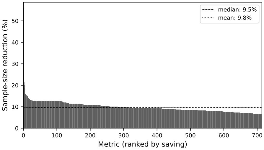
Setting the total sample size to k · n_z, where k^(α, β, t0) is the closed-form correction factor and n_z is the fixed-sample size for a given allocation ratio, produces empirical power within approximately 3 percentage points of the target in Gaussian simulations across the three examined boundaries.
What carries the argument
The correction factor k^(α, β, t0) computed from elementary functions and the bivariate normal CDF using only the boundary value and slope at the planned endpoint.
If this is right
- The correction applies to any smooth concave boundary because it uses only the endpoint value and slope.
- The factor depends on the allocation ratio solely through the burn-in fraction t0.
- The adjustment saves 8 to 20 percent of the sample budget required by the last-point rule across the operating range.
- Sensitivity to the burn-in parameter can be checked directly from the closed-form expression.
Where Pith is reading between the lines
- Experimentation platforms could replace per-metric simulation loops with direct evaluation of the correction factor.
- The same endpoint-slope reduction might be tested on boundaries arising from other always-valid constructions beyond the three cases examined.
- The dependence on t0 alone suggests the correction could be tabulated once per burn-in fraction and reused across metrics.
Load-bearing premise
The closed-form approximation depends on the boundary only through its value and slope at the planned endpoint.
What would settle it
Running the same power simulations with non-Gaussian data or with boundaries that deviate strongly from smoothness and concavity at the endpoint would show whether the achieved power stays inside the reported 3-percentage-point window.
Figures
read the original abstract
Sequential tests that allow continuous monitoring are common in A/B experimentation. Power calculations for these tests require simulations that are hard to scale across many metrics on an experimentation platform. Instead, a common sizing heuristic inflates the fixed-sample size until the marginal rejection probability at the planned endpoint reaches $1-\beta$. This last-point rule is conservative because always-valid (AV) power is the probability of a boundary crossing at any time during the run, not at the endpoint alone. We give a closed-form correction factor $k^(\alpha, \beta, t_0)$ expressed in elementary functions and the bivariate normal CDF, where $t_0 = m/n_z$ is the burn-in fraction. The closed-form approximation depends on the boundary only through its value and slope at the planned endpoint and can be evaluated for any smooth concave boundary. We work out three cases: the confidence sequences of Waudby-Smith et al. (2023) and Maharaj et al. (2023), and the mixture sequential probability ratio test of Johari et al. (2022). Setting the total sample size to $k^ \cdot n_z$, where $n_z$ is the fixed-sample size for allocation ratio $r$, hits empirical power within approximately 3 percentage points of target in Gaussian simulations. The correction factor depends on the allocation ratio $r$ only through $t_0 = m/n_z(r)$. We study sensitivity to the burn-in parameter and show that the correction saves 8--20% of the last-point sample budget across the operating range.
Editorial analysis
A structured set of objections, weighed in public.
Referee Report
Summary. The manuscript claims a closed-form correction factor k^(α, β, t0) expressed via elementary functions and the bivariate normal CDF that adjusts the fixed-sample size n_z (for allocation ratio r) to k · n_z so that always-valid power reaches the target 1-β. The factor depends on any smooth concave boundary only through its value and slope at the planned endpoint t0 = m/n_z; explicit forms are derived for the Waudby-Smith et al. (2023), Maharaj et al. (2023), and Johari et al. (2022) boundaries. Gaussian simulations are reported to recover target power within approximately 3 percentage points, with 8–20% sample-budget savings relative to the last-point rule.
Significance. If the endpoint-reduction approximation holds with the stated accuracy, the result supplies a practical, simulation-free sizing tool for always-valid sequential tests that scales across metrics on experimentation platforms. The closed-form character, the explicit scoping to boundary value and slope at the endpoint, and the reported sample savings are concrete strengths.
major comments (2)
- [Abstract] Abstract: the claim that the correction 'hits empirical power within approximately 3 percentage points of target in Gaussian simulations' is presented without reported simulation count, standard errors, or confidence intervals, so the precision and robustness of the 3pp figure cannot be assessed from the given information.
- [paragraph on the correction factor] The central modeling step (abstract, paragraph on the correction factor) reduces any smooth concave boundary to its value and slope at the endpoint; the manuscript supplies no analytic error bound on this reduction and asserts accuracy solely via the three empirical cases, which is load-bearing for the closed-form claim.
minor comments (2)
- The dependence of k on the allocation ratio r is stated to occur only through t0 = m/n_z(r); an explicit one-line expression or table entry showing this substitution would improve clarity.
- [Abstract] The abstract mentions sensitivity analysis to the burn-in parameter but does not indicate whether the reported 8–20% savings remain stable when t0 varies over the full operating range examined.
Simulated Author's Rebuttal
We thank the referee for the positive evaluation and the recommendation for minor revision. We address each major comment below.
read point-by-point responses
-
Referee: [Abstract] Abstract: the claim that the correction 'hits empirical power within approximately 3 percentage points of target in Gaussian simulations' is presented without reported simulation count, standard errors, or confidence intervals, so the precision and robustness of the 3pp figure cannot be assessed from the given information.
Authors: We agree that the abstract would benefit from including the simulation count, standard errors, and confidence intervals to allow readers to assess the precision of the reported accuracy. We will revise the abstract to incorporate these details from the simulation study presented in the main text. revision: yes
-
Referee: [paragraph on the correction factor] The central modeling step (abstract, paragraph on the correction factor) reduces any smooth concave boundary to its value and slope at the endpoint; the manuscript supplies no analytic error bound on this reduction and asserts accuracy solely via the three empirical cases, which is load-bearing for the closed-form claim.
Authors: The reduction of any smooth concave boundary to its value and slope at the endpoint is a deliberate modeling approximation that enables the closed-form expression via the bivariate normal CDF. Its accuracy is characterized through the Gaussian simulations for the three boundary families rather than an analytic error bound, which we do not supply. We will add a clarifying sentence in the revised manuscript noting the empirical nature of the validation for this approximation. revision: partial
Circularity Check
No significant circularity identified
full rationale
The derivation presents a closed-form correction k^(α, β, t0) obtained from the bivariate normal CDF together with the boundary value and slope evaluated only at the planned endpoint. This construction is scoped explicitly to smooth concave boundaries and is validated by direct Gaussian simulation rather than by fitting parameters to the target power or by reducing to any self-citation chain. No equation in the provided text equates a claimed prediction to a fitted input or to a prior result whose justification loops back to the present paper; the central claim therefore remains independent of its own outputs.
Axiom & Free-Parameter Ledger
axioms (2)
- standard math Bivariate normal CDF accurately captures the joint distribution of the test statistic at burn-in and at the planned endpoint under optional stopping.
- domain assumption Any smooth concave boundary can be approximated for power purposes by its value and slope at the planned endpoint.
Reference graph
Works this paper leans on
-
[1]
doi: 10.24033/asens.476. Patrick Billingsley.Convergence of Probability Measures. John Wiley & Sons,
-
[2]
Sequential testing (documentation).https://docs.growthbook.io/statistics/ sequential
GrowthBook. Sequential testing (documentation).https://docs.growthbook.io/statistics/ sequential. accessed 2026-05-06. Steven R. Howard, Aaditya Ramdas, Jon McAuliffe, and Jasjeet Sekhon. Time-uniform, nonpara- metric, nonasymptotic confidence sequences.The Annals of Statistics, 49(2):1055–1080,
2026
-
[3]
doi: 10.1214/20-AOS1991. Ramesh Johari, Pete Koomen, Leonid Pekelis, and David J. Walsh. Always valid inference: continuous monitoring of A/B tests.Operations Research, 70(3):1806–1821,
-
[4]
Operations Research , author =
doi: 10.1287/opre.2021.2135. Akash Maharaj, Ritwik Sinha, David Arbour, Ian Waudby-Smith, Simon Z. Liu, Moumita Sinha, Raghavendra Addanki, Aaditya Ramdas, Manas Garg, and Viswanathan Swaminathan. Anytime-valid confidence sequences in an enterprise A/B testing platform. InCompanion Pro- ceedings of the ACM Web Conference 2023 (WWW ’23 Companion),
-
[5]
doi: 10.1145/3543873. 3584635. 8 Herbert Robbins and David Siegmund. Boundary crossing probabilities for the Wiener process and sample sums.The Annals of Mathematical Statistics, 41(5):1410–1429,
-
[6]
doi: 10.1214/aoms/ 1177696787. M˚ arten Schultzberg. Nobody puts Bonferroni in a corner.arXiv preprint,
-
[7]
M˚ arten Schultzberg, Sebastian Ankargren, and Mattias Fr˚ anberg
arXiv:2604.09256. M˚ arten Schultzberg, Sebastian Ankargren, and Mattias Fr˚ anberg. Risk-aware product decisions in A/B tests with multiple metrics.Journal of Statistical Planning and Inference, 245:106393,
-
[8]
David Siegmund.Sequential Analysis: Tests and Confidence Intervals
doi: 10.1093/biomet/64.2.177. David Siegmund.Sequential Analysis: Tests and Confidence Intervals. Springer-Verlag,
-
[9]
Ian Waudby-Smith, Edward H. Kennedy, and Aaditya Ramdas. Distribution-uniform anytime-valid sequential inference and the Robbins-Siegmund distributions.arXiv:2311.03343,
-
[10]
The proof uses the WSKR boundary as the worked example; the Maharaj boundary follows by substitutingb M(k) andb ′ M(k) forb W(k) andb ′ W(k) in the final expressions
A Derivation ofk ∗ The derivation strategy (tangent linearisation of a curved boundary, Bachelier first-passage on the linear surrogate, integration over the initial value) follows Siegmund [1977], applied here to the specific boundary families arising in modern confidence sequences. The proof uses the WSKR boundary as the worked example; the Maharaj boun...
1977
-
[11]
yieldsϱ 2/(1+ϱ)2 < 4 log2(1+ϱ), soφ(ϱ)<0 andb M is strictly concave on [t 0,∞). A.2. Linearisation.Replacebon [t 0, k] by its tangent att=k: L(t) =b(k) +s(t−k), s=b ′(k), L t0 =b(k)−s(k−t 0).(17) A.3. Bachelier first-passage on the linear boundary.The classical Bachelier formula for Brownian motionW t with driftµand variance rate 1 states that for a linea...
1900
-
[12]
The right-hand side of (20) follows
Standardising the second component gives correlation−B 0/ p 1 +B 2 0, and the joint event{u≤c, V−B 0u≤A 0}becomes{u≤c, fW≤A 0/ p 1 +B 2 0}with fWunit variance. The right-hand side of (20) follows. Applying Lemma 1 to the first term of (18) withA 0 =ν √ T− √t0 cx/ √ TandB 0 = √t0/ √ T yields (12) after the substitutions 1 +B 2 0 = (T+t 0)/T,A 0/ p 1 +B 2 0...
2000
discussion (0)
Sign in with ORCID, Apple, or X to comment. Anyone can read and Pith papers without signing in.