pith. sign in

arxiv: 2606.20509 · v1 · pith:A23MLKNBnew · submitted 2026-06-18 · 🧮 math.DS

Planar constant piecewise smooth vector fields with large hysteresis

Pith reviewed 2026-06-26 15:18 UTC · model grok-4.3

classification 🧮 math.DS
keywords piecewise smooth vector fieldshysteresislimit setsplanar systemsswitching boundarieslinear vector fieldscontrol systemsdynamical systems
0
0 comments X

The pith

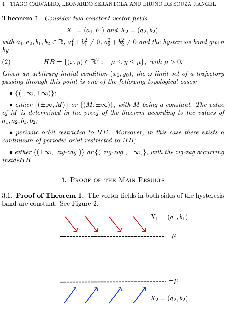
Planar systems with two linear vector fields and hysteresis switching between two boundaries begin classification of their limit sets.

A machine-rendered reading of the paper's core claim, the machinery that carries it, and where it could break.

The paper addresses the lack of mathematical classification for limit sets in control systems that switch between vector fields based on thresholds, such as disease treatment protocols that pause when cell levels drop below one value and resume above another. It initiates this classification effort by restricting attention to the planar case using exactly two linear vector fields separated by two switching boundaries. A sympathetic reader would care because these switched models appear in applications yet have no established theory for what long-term behaviors, such as convergence to equilibria or periodic orbits, can occur. If the planar analysis succeeds, it supplies the starting point for determining the possible attractors under the hysteresis rule.

Core claim

The authors establish that the planar case with two linear vector fields active across two switching boundaries under large hysteresis provides a tractable setting in which the limit sets of the resulting dynamics can be determined rigorously, serving as the foundation for a broader classification of such models.

What carries the argument

The planar hysteresis switching system consisting of two linear vector fields separated by two boundaries that trigger the switch when trajectories cross the thresholds.

Load-bearing premise

Analysis of the restricted planar case with two linear vector fields and two switching boundaries yields a classification whose structure extends to more general hysteresis models without fundamental alteration.

What would settle it

A specific planar example with two linear vector fields and two hysteresis thresholds whose observed long-term behavior falls outside the limit-set categories obtained from the planar analysis.

Figures

Figures reproduced from arXiv: 2606.20509 by Bruno de Souza Rangel, Leonardo Serantola, Tiago Carvalho.

Figure 1
Figure 1. Figure 1: The configuration studied with an hysteresis band HB between y = −µ and y = µ. The vector field X1 acts on the region Σ+ and the vector field X2 acts on the region Σ−. Remark 1. IMPORTANT CONVENTION: In this paper we will con￾sider that when an initial condition of a solution belongs to HB, then the vector field to be considered is X2. Physically, we are thinking that in HB the ”treatment” X1 is not applie… view at source ↗
Figure 2
Figure 2. Figure 2: An example of two constant vector fields acting in the upper region and the down region of the hysteresis band with b1 < 0 and a1, a2, b2 > 0. Here we will analyze the dynamics for all cases where a1 > 0 and b1 = 0. See [PITH_FULL_IMAGE:figures/full_fig_p004_2.png] view at source ↗
Figure 3
Figure 3. Figure 3: Dynamics for conditions a1 > 0 and b1 = 0. • Case 1.12: a1 < 0, b1 = 0, a2 < 0, b2 > 0. Given an arbitrary initial condition (x0, y0), the trajectory has ω-limit set {(−∞, y0)} when y0 > µ and has ω-limit set {(−∞, µ)} when y0 ≤ µ. • Case 1.13: a1 < 0, b1 = 0, a2 < 0, b2 = 0. Given an arbitrary initial condition (x0, y0), the trajectory has ω-limit set {(−∞, y0)}. • Case 1.14: a1 < 0, b1 = 0, a2 < 0, b2 < … view at source ↗
Figure 4
Figure 4. Figure 4: Bifurcation diagram in the variables a2 and b2, for a1 > 0 and b1 = 0. • Case 1.16: a1 < 0, b1 = 0, a2 > 0, b2 < 0. Given an arbitrary initial condition (x0, y0), the trajectory has ω-limit set {(−∞, y0)} when y0 > µ and has ω-limit set {(+∞, −∞)} when y0 ≤ µ. Here we will analyze the dynamics for all cases where a1 = 0 and b1 > 0. See [PITH_FULL_IMAGE:figures/full_fig_p007_4.png] view at source ↗
Figure 5
Figure 5. Figure 5: Dynamics for conditions a1 < 0 and b1 = 0. when y0 > µ and has ω-limit set x0 + a2(−y0 + µ) b2 , +∞  , when y0 ≤ µ • Case 1.21: a1 = 0, b1 > 0, a2 < 0, b2 = 0. In this case, taking an arbitrary initial condition (x0, y0), the trajectory has ω-limit set {(x0, +∞)} when y0 > µ and has ω-limit set {(−∞, y0)} when y0 ≤ µ. • Case 1.22: a1 = 0, b1 > 0, a2 < 0, b2 < 0. In this case, taking an arbitrary initia… view at source ↗
Figure 6
Figure 6. Figure 6: Bifurcation diagram in the variables a2 and b2, for a1 < 0 and b1 = 0. • Case 1.23: a1 = 0, b1 > 0, a2 = 0, b2 < 0. In this case, taking an arbitrary initial condition (x0, y0), the trajectory has ω-limit set {(x0, +∞)} when y0 > µ and has ω-limit set {(x0, −∞)} when y0 ≤ µ. • Case 1.24: a1 = 0, b1 > 0, a2 > 0, b2 < 0. In this case, taking an arbitrary initial condition (x0, y0), the trajectory has ω-limit… view at source ↗
Figure 7
Figure 7. Figure 7: Dynamics for conditions a1 = 0 and b1 > 0. • Case 1.30: a1 = 0, b1 < 0, a2 < 0, b2 < 0. In this case, taking an arbi￾trary initial condition (x0, y0), the trajectory has ω-limit set {(−∞, −∞)}. • Case 1.31: a1 = 0, b1 < 0, a2 = 0, b2 < 0. In this case, taking an arbitrary initial condition (x0, y0), the trajectory has ω-limit set {(x0, −∞)} [PITH_FULL_IMAGE:figures/full_fig_p010_7.png] view at source ↗
Figure 8
Figure 8. Figure 8: Bifurcation diagram in the variables a2 and b2, for a1 = 0 and b1 > 0. • Case 1.32: a1 = 0, b1 < 0, a2 > 0, b2 < 0. In this case, taking an arbi￾trary initial condition (x0, y0), the trajectory has ω-limit set {(+∞, −∞)}. Here we will analyze the dynamics for all cases where a1 > 0 and b1 > 0. See [PITH_FULL_IMAGE:figures/full_fig_p011_8.png] view at source ↗
Figure 9
Figure 9. Figure 9: Dynamics for conditions a1 = 0 and b1 < 0. • Case 1.39: a1 > 0, b1 > 0, a2 = 0, b2 < 0. In this case, taking an arbi￾trary initial condition (x0, y0), the trajectory has ω-limit set {(+∞, +∞)} when y0 > µ and has ω-limit set {(x0, −∞)} when y0 ≤ µ [PITH_FULL_IMAGE:figures/full_fig_p012_9.png] view at source ↗
Figure 10
Figure 10. Figure 10: Bifurcation diagram in the variables a2 and b2, for a1 = 0 and b1 < 0. • Case 1.40: a1 > 0, b1 > 0, a2 > 0, b2 < 0. In this case, taking an arbi￾trary initial condition (x0, y0), the trajectory has ω-limit set {(+∞, +∞)} when y0 > µ and has ω-limit set {(+∞, −∞)} when y0 ≤ µ. Here we will analyze the dynamics for all cases where a1 > 0 and b1 < 0. See [PITH_FULL_IMAGE:figures/full_fig_p013_10.png] view at source ↗
Figure 11
Figure 11. Figure 11: Dynamics for conditions a1 > 0 and b1 > 0. • Case 1.47: a1 > 0, b1 < 0, a2 = 0, b2 < 0. In this case, taking an arbitrary initial condition (x0, y0), the trajectory has ω-limit set x0 + a1(−y0 + µ) b1 , −∞ , when y0 > µ and has ω-limit set {(x0, −∞)} when y0 ≤ µ. • Case 1.48: a1 > 0, b1 < 0, a2 > 0, b2 < 0. In this case, taking an arbi￾trary initial condition (x0, y0), the trajectory has ω-limit set {… view at source ↗
Figure 12
Figure 12. Figure 12: Bifurcation diagram in the variables a2 and b2, for a1 > 0 and b1 > 0. Here we will analyze the dynamics for all cases where a1 < 0 and b1 > 0. See [PITH_FULL_IMAGE:figures/full_fig_p015_12.png] view at source ↗
Figure 13
Figure 13. Figure 13: Dynamics for conditions a1 > 0 and b1 < 0. • Case 1.56: a1 < 0, b1 > 0, a2 > 0, b2 < 0. In this case, taking an arbi￾trary initial condition (x0, y0), the trajectory has ω-limit set {(−∞, +∞)} when y0 > µ and has ω-limit set {(+∞, −∞)} when y0 ≤ µ. Here we will analyze the dynamics for all cases where a1 < 0 and b1 < 0. See [PITH_FULL_IMAGE:figures/full_fig_p016_13.png] view at source ↗
Figure 14
Figure 14. Figure 14: Bifurcation diagram in the variables a2 and b2, for a1 > 0 and b1 < 0. • Case 1.57: a1 < 0, b1 < 0, a2 > 0, b2 = 0. In this case, taking an arbitrary initial condition (x0, y0), the trajectory has ω-limit set {(+∞, µ)} when y0 > µ and has ω-limit set {(+∞, y0)} when y0 ≤ µ. • Case 1.58: a1 < 0, b1 < 0, a2 > 0, b2 > 0. To analyze the dynamics of the trajectories, we will use Poincar´e first return map. See… view at source ↗
Figure 15
Figure 15. Figure 15: Dynamics for conditions a1 < 0 and b1 > 0. 3.1.1. Poincar´e first return map. In this section, via the Poincar´e first return map, let us describe the dynamics of the trajectories of X1 and X2 in the cases 1.26, 1.27, 1.28, 1.42, 1.43, 1.44, 1.58, 1.59, 1.60. Note that b1b2 ̸= 0. Let us suppose an initial point p1 = [PITH_FULL_IMAGE:figures/full_fig_p018_15.png] view at source ↗
Figure 16
Figure 16. Figure 16: Bifurcation diagram in the variables a2 and b2, for a1 < 0 and b1 > 0. The time which the flow takes to reach the another boundary of the hys￾teresis band y = −µ is given by (3) t = − 2µ b1 . Substituting (3) in the component solution x1 gives us x1  − 2µ b1  := x 2 0 = x 1 0 − 2a1µ b1 . From this moment, the flow is governed by the vector field X2 located under the hysteresis region and the solutions f… view at source ↗
Figure 17
Figure 17. Figure 17: Dynamics for conditions a1 < 0 and b1 < 0. with b1b2 ̸= 0. Therefore, if α = 0, the Poincar´e first return map presents infinite fixed points located at the line [PITH_FULL_IMAGE:figures/full_fig_p020_17.png] view at source ↗
Figure 18
Figure 18. Figure 18: Bifurcation diagram in the variables a2 and b2, for a1 < 0 and b1 < 0. x-coordinate going to −∞. The cases that represent α < 0 are the cases 1.44, 1.58 when a2/b2 < a1/b1 and the cases 1.28, 1.59, 1.60. See [PITH_FULL_IMAGE:figures/full_fig_p021_18.png] view at source ↗
Figure 19
Figure 19. Figure 19: Possible cases when α = 0. A particularly interesting result is that the existence of periodic orbits and monotone zig-zag dynamics can be determined by a simple parameter involving the slopes of the two vector fields. This provides a clear geometric interpretation of the mechanisms responsible for the long-term behavior of the system. The present work should be regarded as a first step toward a broader t… view at source ↗
read the original abstract

Throughout this work, we will carry out a rigorous mathematical analysis of a class of control systems that is widely used in applications but still lacks a consistent theoretical foundation for describing the types of limit sets that may arise from its dynamics. There are applications in which, for example, a treatment for a given disease is administered until the level of diseased cells falls below a prescribed threshold C1. At that point, the treatment is suspended in order to allow the patient's organism to recover from its side effects. Subsequently, when the level of diseased cells reaches a second threshold C2 bigger than C1, the treatment is resumed, and the protocol is repeated. To the best of our knowledge, there is not a mathematical classification of such models. In this paper, we initiate what is intended to become a consistent body of literature aimed at determining the limit sets of such models. We begin with the planar case, in which two linear vector fields are active and two switching boundaries are considered. Naturally, in future developments, control systems in higher dimensions, featuring additional vector fields and more general switching manifolds, should also be considered.

Editorial analysis

A structured set of objections, weighed in public.

Desk editor's note, referee report, simulated authors' rebuttal, and a circularity audit. Tearing a paper down is the easy half of reading it; the pith above is the substance, this is the friction.

Referee Report

1 major / 0 minor

Summary. The manuscript states an intention to carry out rigorous mathematical analysis of planar constant piecewise-smooth vector fields with large hysteresis and to begin classifying their limit sets. It restricts attention to the case of exactly two linear vector fields and two switching boundaries, motivated by applications such as threshold-based treatment protocols, and positions this planar setting as the starting point for a larger research program on such systems.

Significance. A delivered classification of limit sets in this restricted planar setting would address the acknowledged absence of a mathematical foundation for a class of hysteresis-based control systems that appear in applications. The choice of two linear fields and two boundaries is presented as a tractable entry point whose qualitative features might extend to higher dimensions and more fields.

major comments (1)
  1. [Abstract] Abstract: The abstract states an intention to perform rigorous analysis and begin classification but supplies no theorems, derivations, or concrete limit-set results; the central claim therefore rests on future work that is not yet shown.

Simulated Author's Rebuttal

1 responses · 0 unresolved

We thank the referee for their review. We respond to the single major comment below.

read point-by-point responses
  1. Referee: [Abstract] Abstract: The abstract states an intention to perform rigorous analysis and begin classification but supplies no theorems, derivations, or concrete limit-set results; the central claim therefore rests on future work that is not yet shown.

    Authors: The manuscript is explicitly an initial contribution that sets up the planar system with two linear fields and two switching boundaries and begins the classification by providing rigorous analysis of trajectories and identification of certain limit sets. We agree, however, that the abstract places greater emphasis on the long-term research program than on the concrete results contained in the paper. In the revised version we will update the abstract to summarize the specific setup, the theorems proved, and the limit sets classified in this work. revision: yes

Circularity Check

0 steps flagged

No significant circularity; paper initiates classification without load-bearing derivations

full rationale

The manuscript explicitly frames its contribution as the start of a new research program rather than a completed derivation or classification. It states the goal of determining limit sets for planar systems with exactly two linear vector fields and two switching boundaries, but provides no equations, fitted parameters, predictions, or uniqueness theorems that reduce to prior self-citations or inputs by construction. The abstract and setup contain no self-definitional steps, fitted-input predictions, or ansatzes smuggled via citation. The work is self-contained as an initial tractable case whose extension is left for future papers.

Axiom & Free-Parameter Ledger

0 free parameters · 0 axioms · 0 invented entities

Abstract-only review supplies no explicit free parameters, axioms, or invented entities.

pith-pipeline@v0.9.1-grok · 5724 in / 1063 out tokens · 15495 ms · 2026-06-26T15:18:35.574809+00:00 · methodology

discussion (0)

Sign in with ORCID, Apple, or X to comment. Anyone can read and Pith papers without signing in.

Reference graph

Works this paper leans on

7 extracted references

  1. [1]

    D. J. W. Simpson , A compendium of Hopf-like bifurcations in piecewise-smooth dynamical systems , Phys. Lett., A 382, No. 35, 2439-2444 (2018)

  2. [2]

    D. J. W. Simpson , Twenty Hopf-like bifurcations in piecewise-smooth dynamical systems , Phys. Rep. 970, 1-80 (2022)

  3. [3]

    Zhang, Jingsong and Cunningham, Jessica and Brown, Joel and Gatenby, Robert , ntegrating evolutionary dynamics into treatment of metastatic castrate-resistant prostate cancer , Nature Communications 8:1816 (2017)

  4. [4]

    e76284 (2022)

    Zhang, Jingsong and Cunningham, Jessica and Brown, Joel and Gatenby, Robert , Evolution-based mathematical models significantly prolong response to abiraterone in metastatic castrate-resistant prostate cancer and identify strategies to further improve outcomes , eLife, 110, p. e76284 (2022)

  5. [5]

    RWA 82, p

    Tiago Carvalho, Jackson Cunha, Rodrigo Euzébio, Marco Florentino , Dynamics of an intermittent HIV treatment using piecewise smooth vector fields with two switching manifolds , Nonlinear Anal. RWA 82, p. 104256 (2025)

  6. [6]

    Buzzi and Tiago Carvalho and Marco A

    Claudio A. Buzzi and Tiago Carvalho and Marco A. Teixeira , Birth of limit cycles bifurcating from a nonsmooth center , J. Math. Pures Appl. 102, p. 36-47 (2014)

  7. [7]

    Li, T-Y.; Yorke, J. A. , Period Three Implies Chaos , The American Mathematical Monthly, v. 82, n. 10, p. 985–992, (1975)