Diffusion-Driven State Space Models
Pith reviewed 2026-06-26 13:14 UTC · model grok-4.3
The pith
Diffusion-Driven State Space Model replaces Gaussian transitions with a diffusion model for joint training on sequential data.
A machine-rendered reading of the paper's core claim, the machinery that carries it, and where it could break.
Core claim
By replacing the conventional Gaussian transition distribution with a diffusion model, the DDSSM resolves the open problem of how to jointly train an autoencoder and a diffusion model on sequential data, thereby extending the literature on latent diffusion models for time series, and it empirically outperforms a state-of-the-art deep SSM at fitting and forecasting a simulated time series with multimodal transitions.
What carries the argument
The diffusion model serving as the transition distribution inside the state space model framework, which enables stable joint optimization with an autoencoder on sequential observations.
If this is right
- State space models can capture non-Gaussian and multimodal latent transitions while retaining tractable inference.
- Latent diffusion models acquire a structured way to model time series through the state space backbone.
- Forecasting improves for systems whose latent dynamics exhibit multiple modes rather than simple Gaussian spread.
- The joint-training procedure extends prior work on autoencoders paired with diffusion processes into the sequential setting.
Where Pith is reading between the lines
- The same replacement of transition distributions could be tested with other expressive generative models beyond diffusion.
- Domains that produce sequential observations with abrupt mode switches, such as sensor streams or financial returns, become natural candidates for the approach if the simulated gains carry over.
- Scaling experiments on longer sequences or higher-dimensional observations would clarify whether the joint training remains stable in more demanding regimes.
Load-bearing premise
The diffusion-based transition integrates into the SSM framework for joint training without creating intractable inference or optimization problems, and that gains on one simulated multimodal series indicate wider usefulness.
What would settle it
A case in which joint training of the autoencoder and diffusion model fails to converge or yields worse forecasts than the Gaussian baseline on additional multimodal time series would show the integration does not work as claimed.
Figures
read the original abstract
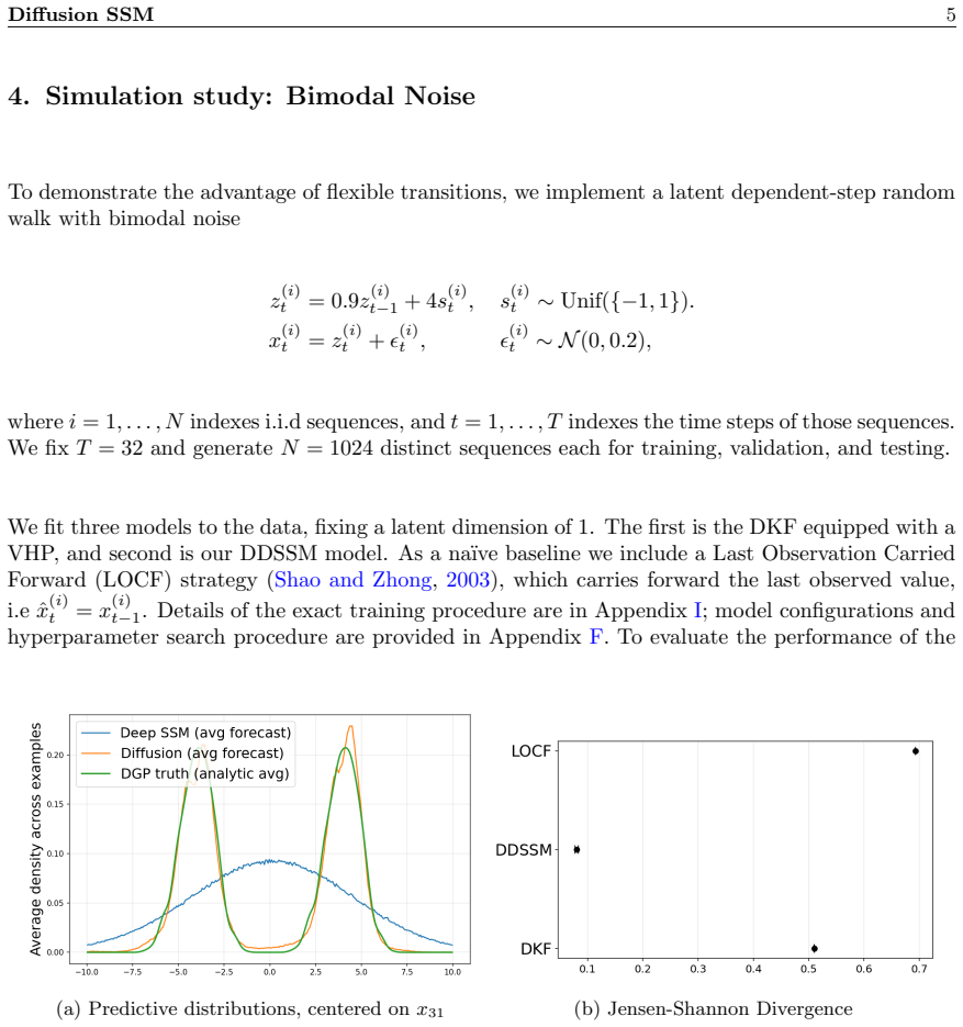
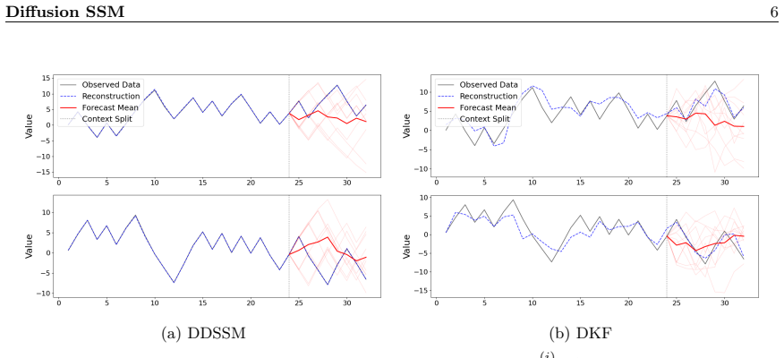
In many domains, practitioners seek models that produce accurate forecasts while faithfully capturing latent system dynamics. Existing approaches typically sacrifice one of these goals: deep state space models often assume Gaussian latent transitions, limiting fit and forecasting, while diffusion models are highly expressive but lack principled inference for the underlying dynamics. To combine the strengths of both, we introduce the Diffusion-Driven State Space Model (DDSSM), which replaces the conventional Gaussian transition distribution with a diffusion model. Our DDSSM resolves the open problem of how to jointly train an autoencoder and a diffusion model on sequential data, thereby extending the literature on latent diffusion models for time series. Moreover, we find that the DDSSM empirically outperforms a state-of-the-art deep SSM at fitting and forecasting a simulated time series with multimodal transitions.
Editorial analysis
A structured set of objections, weighed in public.
Referee Report
Summary. The manuscript introduces the Diffusion-Driven State Space Model (DDSSM), which replaces the conventional Gaussian transition distribution in state space models with a diffusion model. It claims to resolve the open problem of jointly training an autoencoder and a diffusion model on sequential data, extending latent diffusion models for time series, and reports that DDSSM empirically outperforms a state-of-the-art deep SSM at fitting and forecasting a simulated time series with multimodal transitions.
Significance. If the claimed joint training procedure proves tractable and the outperformance result holds under standard controls, the work would usefully combine the expressiveness of diffusion transitions with the inference structure of SSMs. The identification of an open joint-training problem and its proposed resolution would constitute a targeted contribution to time-series latent variable modeling.
major comments (1)
- [Abstract] Abstract: the empirical outperformance claim over a state-of-the-art deep SSM is asserted without any description of methods, metrics, baselines, error bars, dataset details, or experimental protocol, so the support for the central claim cannot be assessed from the available text.
Simulated Author's Rebuttal
We thank the referee for their review and for identifying the need for clearer experimental context around our central empirical claim. We address the comment below.
read point-by-point responses
-
Referee: [Abstract] Abstract: the empirical outperformance claim over a state-of-the-art deep SSM is asserted without any description of methods, metrics, baselines, error bars, dataset details, or experimental protocol, so the support for the central claim cannot be assessed from the available text.
Authors: We agree that the abstract, by design, is a concise summary and does not contain the experimental details. The full manuscript provides these in Section 4 (experimental setup, including the simulated multimodal time series, baselines, metrics such as negative log-likelihood and forecast error, error bars from multiple runs, and protocol) and Section 5 (results). The abstract follows standard practice of highlighting the claim while deferring details to the body. To improve accessibility, we will revise the abstract to include a brief clause referencing the evaluation on simulated data with multimodal transitions and comparison to deep SSM baselines. revision: yes
Circularity Check
No significant circularity detected
full rationale
The abstract and available description introduce the DDSSM model and report an empirical outperformance on one simulated multimodal time series, but contain no equations, derivations, fitted parameters presented as predictions, or self-citations that reduce any claim to its inputs by construction. The central claims rest on model introduction and empirical results rather than any self-referential fitting or uniqueness theorem imported from prior author work. This is the expected honest non-finding for a high-level description lacking load-bearing technical steps.
Axiom & Free-Parameter Ledger
Reference graph
Works this paper leans on
-
[1]
Training deep nets with sublinear memory cost.arXiv preprint arXiv:1604.06174,
Tianqi Chen, Bing Xu, Chiyuan Zhang, and Carlos Guestrin. Training deep nets with sublinear memory cost.arXiv preprint arXiv:1604.06174,
-
[2]
Maximilian Karl, Maximilian Soelch, Justin Bayer, and Patrick Van der Smagt. Deep varia- tional bayes filters: Unsupervised learning of state space models from raw data.arXiv preprint arXiv:1605.06432,
-
[3]
Deep kalman filters.arXiv preprint arXiv:1511.05121,
Rahul G Krishnan, Uri Shalit, and David Sontag. Deep kalman filters.arXiv preprint arXiv:1511.05121,
-
[4]
Auto-encoding sequential monte carlo.arXiv preprint arXiv:1705.10306,
Tuan Anh Le, Maximilian Igl, Tom Rainforth, Tom Jin, and Frank Wood. Auto-encoding sequential monte carlo.arXiv preprint arXiv:1705.10306,
-
[5]
Jian Qian, Bingyu Xie, Biao Wan, Minhao Li, Miao Sun, and Patrick Yin Chiang. Timeldm: Latent diffusion model for unconditional time series generation.arXiv preprint arXiv:2407.04211,
-
[6]
Taming vaes.arXiv preprint arXiv:1810.00597,
Danilo Jimenez Rezende and Fabio Viola. Taming vaes.arXiv preprint arXiv:1810.00597,
-
[7]
Yang Song, Jascha Sohl-Dickstein, Diederik P Kingma, Abhishek Kumar, Stefano Ermon, and Ben Poole. Score-based generative modeling through stochastic differential equations.arXiv preprint arXiv:2011.13456,
Pith/arXiv arXiv 2011
-
[8]
Diffusion models for time series forecasting: A survey.arXiv preprint arXiv:2507.14507,
Chen Su, Zhengzhou Cai, Yuanhe Tian, Zhuochao Chang, Zihong Zheng, and Yan Song. Diffusion models for time series forecasting: A survey.arXiv preprint arXiv:2507.14507,
-
[9]
State Space Model Derivation A.1
Diffusion SSM 11 A. State Space Model Derivation A.1. Derivation of the Generative Model Our goal is to learn a model of the conditional distributionp(x 1:T |u1:T ). Following the general framework of Girin et al. (2022), we introduce a sequence of latent variablesz 1:T = (z1,z 2, . . . ,zT ), where eachz t ∈R d is ad-dimensional vector, and factorize the...
2022
-
[10]
jY t=1 p(zt |x t:T ,z 1:t−1,u 1:t) # ·
and train under the VAE framework which allows jointly learning the generative model and the inference model. The primary objective is to maximize the marginal log-likelihood logp(x 1:T |u1:T ) with respect to the parameters of the generative model. As is typical with latent-variable models, exact inference depends on the smoothing posterior distribution ...
2022
-
[11]
−log p(t) ψ (z0:K−1 t |zK t ,c t)p(zK t ) q(z1:K t |z0 t ) # (29c) =E q(z1:K t |z0 t)
and other works on deep state-space models (Girin et al., 2022). To implement this dependence, we follow Krishnan et al. (2017) and employ a neural-network to summarize the future observationsx t:T for each timesteptinto a fixed-dimensional vectorh t. We define (hT ,h T−1 , . . .h1) =F ϕ(concat(x1:T )) (21) The implementation ofF ϕ used by Krishnan et al....
2022
-
[12]
To recover our original objective, we use thatϵ= ˆzk t −z0 t σk to recover the predicted noise, ϵψ ˜zk t , k,c t = ˆzk t −D ψ(ˆzk t , σk,c t) σk
For reference, these coefficients are cskip(σk) = 1 σ2 k + 1, c out(σk) = σkp σ2 k + 1 , cin(σk) = 1p σ2 k + 1 , c noise(σk) = 1 4 log(σk). To recover our original objective, we use thatϵ= ˆzk t −z0 t σk to recover the predicted noise, ϵψ ˜zk t , k,c t = ˆzk t −D ψ(ˆzk t , σk,c t) σk . We now may find a new form for the noise prediction error term in Eq. ...
2021
-
[13]
Parameter Tuning Range DKF DDSSM lambda schedule linear, cosine cosine cosine lambda warmup steps 200 – 1200 867 889 lambda end 0.3 – 2 1.245 1.243 enc lr 5×10 −5 – 10−2 (log) 0.00887 0.000864 dec lr 5×10 −5 – 10−2 (log) 0.00777 0.000300 trans lr 5×10 −5 – 10−2 (log) 0.000099 0.00941 zinit lr 10−4 – 10−3 (log) 0.005 0.000801 S 1 – 4 2 2 batch size 64, 128...
2021
-
[14]
Typically, the prior is chosen by DSSMs to be a standard Gaussian Krishnan et al
in thej= 1 case. Typically, the prior is chosen by DSSMs to be a standard Gaussian Krishnan et al. (2015, 2017); Karl et al. (2016). The prior overz 1 however regularizes the rest of the latent trajectory, as both the transition model and the encoder posterior are conditioned onz
2015
-
[15]
(2019, 2021), where it is demonstrated that a more flexible prior over the initial latent state can lead to better inference about the latent trajectory
This is experimentally validated by Klushyn et al. (2019, 2021), where it is demonstrated that a more flexible prior over the initial latent state can lead to better inference about the latent trajectory. As our diffusion transition model can be highly expressive, we wish to avoid inhibiting the expres- siveness of the transition model by imposing a simpl...
2019
-
[16]
EqΦ(z−j+1:0 |z1:j)
=E p(x1:T )[qϕ(z1|x1:T )]. Diffusion SSM 25 We generalize this to thej-order Markovian setting by introducingjauxiliary variablesz −j+1:0. The conditional distributionp η(z1:j|z−j+1:0) is given by the chain rule, pη(z1:j|z−j+1:0) = jY t=1 pη(zt|zt−1, . . . ,z−j+1) = jY t=1 pη(zt|zt−j:t−1), where we have used thej-order Markovian property in the second lin...
2021
-
[17]
The residual block itself is mostly unchanged from CSDI, except we abstract the time-mixing and feature-mixing operations
and produces an output of the same shape as well as a skip connection. The residual block itself is mostly unchanged from CSDI, except we abstract the time-mixing and feature-mixing operations. This allows us to replace computationally heavy attention operations with architectures like a 1D convolution stack or a Gated Recurrent Unit (GRU) when the sequen...
2021
-
[18]
Future Summary ModuleThe Future Summary module computesh 1:T =F ϕ(x1:T ,m obs). At each time step across the length-Tsequence, we concatenate the observationsx t, absolute time embeddings, observation missingness masksm obs,t, and the flattened static covariates. This feature vector is linearly projected to a hidden dimensionC summary. In line with Krishn...
2017
-
[19]
By placing the future summary at the beginning of the sequence, we allow the Context producer to attend to the future summary at each layer of its architecture
j. By placing the future summary at the beginning of the sequence, we allow the Context producer to attend to the future summary at each layer of its architecture. This choice is once again inspired by Krishnan et al. (2017), who project the future summary to the initial hidden state of their RNN-based encoder, which allows the future summary to influence...
2017
-
[20]
t−1 for the history slots
slots: timetfor the summary slot, andt−j . . . t−1 for the history slots. •Role Mask:We employ a binary mask—set to 0 for the future summary slot and 1 for the history slots—which is projected through a learned linear layer. This explicitly instructs the residual blocks to treat the two modalities differently. •Padding Mask:We use an additional binary mas...
2017
-
[21]
It is only during sampling that we lose parallelism across time steps, in which case the total diffusion cost becomesO(K×T×g(M×j+ 1)), forKdiffusion steps
Therefore given enough memory, the diffusion-incurred time complexity for a forward pass of Algorithm 1 isO(g(M×j+ 1)) wheregis the time complexity of a pass through the diffusion model. It is only during sampling that we lose parallelism across time steps, in which case the total diffusion cost becomesO(K×T×g(M×j+ 1)), forKdiffusion steps. J. Extended Re...
2022
-
[22]
Karl et al. (2016) observed the shortcoming of Gaussian transitions in the context of modeling physical systems, arguing that the regularization provided by Gaussian transitions harms reconstruction performance. Several lines of work have attempted to make the DKF more expressive. Karl et al. (2016) proposed learning a more flexible transition by learning...
2016
-
[23]
Klushyn et al
introduces parametersa 1:T and propose the generative modelp(x 1:T ,a 1:T ,z 1:T |u1:T ) =p(x 1:T |a1:T )p(a1:T |z1:T )p(z1:T |u1:T ), relying on linear Gaussianp(a t|zt,u t) andp(z t|zt−1,h t,u t) distributions. Klushyn et al. (2021) extends this model to have nonlinear Gaussian transitions, proposing the Extended Kalman VAE (EKVAE). The primary advantag...
2021
-
[24]
This is important since the gradients of the diffusion model are used to train the VAE
of the denoising model to reduce the variance of the gradients across noise levels. This is important since the gradients of the diffusion model are used to train the VAE. Details of our approach to concurrent training are described in Appendix E. Latent diffusion models for temporal data. (WIP)Qian et al. (2024) propose a latent diffusion model framework...
2024
discussion (0)
Sign in with ORCID, Apple, or X to comment. Anyone can read and Pith papers without signing in.