Time-domain anomalies in solar and stellar flares
Pith reviewed 2026-06-26 07:15 UTC · model grok-4.3
The pith
A new anomaly index applied to flare catalogs shows that 66 percent of stellar flares and up to 57 percent of solar flares deviate from standard light-curve shapes.
A machine-rendered reading of the paper's core claim, the machinery that carries it, and where it could break.
Core claim
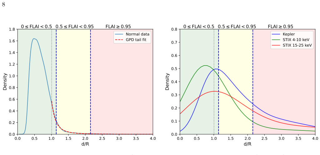
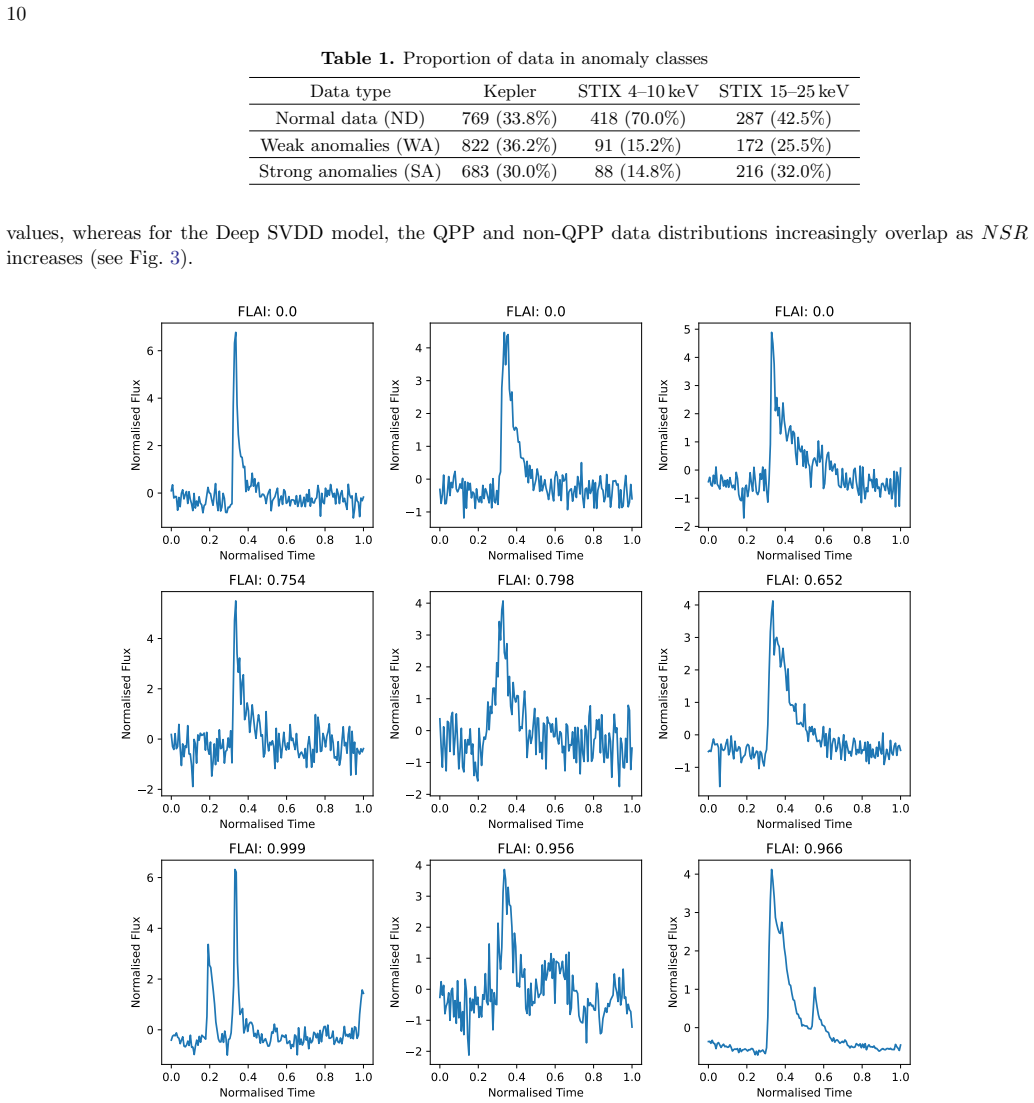
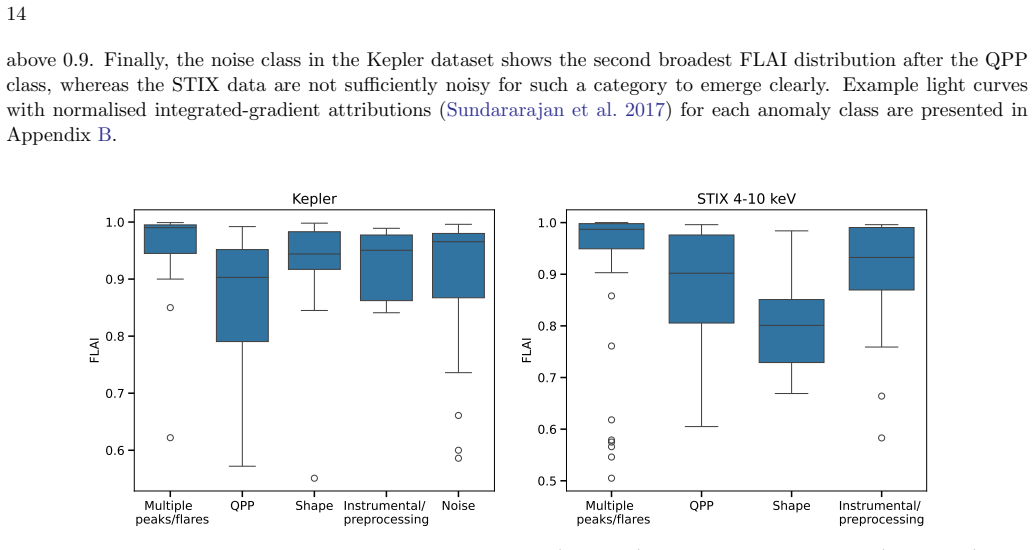
Application of the Flare Anomaly Index to the Kepler white-light catalog classifies 36 percent of events as weak anomalies and 30 percent as strong anomalies, while the same index applied to M- and X-class solar flares from the STIX list classifies 25 percent and 32 percent of events in the 15-25 keV channel as weak and strong anomalies respectively, versus 15 percent for each class in the 4-10 keV channel; the results indicate that anomalous flares occur more often at higher energies and that both solar and stellar flares commonly deviate from the normal population used in model training.
What carries the argument
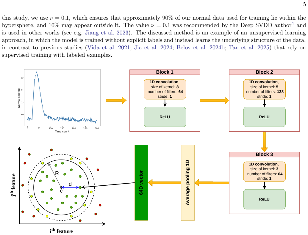
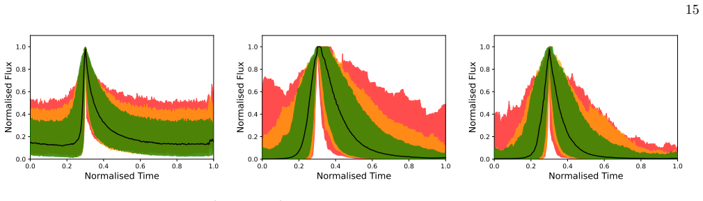
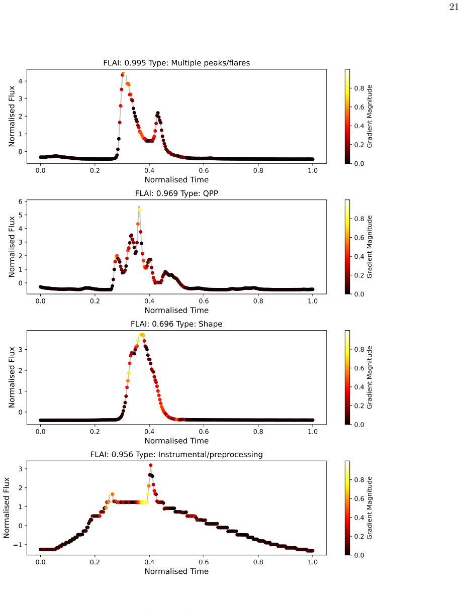
The Flare Anomaly Index (FLAI), a probabilistic score produced by a Deep Support Vector Data Description model trained exclusively on synthetic light curves from analytical flare trend models plus noise, which measures how far an observed light curve lies from the learned distribution of normal flares.
If this is right
- Anomalous flares appear more frequently in the higher-energy STIX channel than in the lower-energy channel.
- Both solar and stellar flares often deviate from the normal flare population used for model training.
- Deviations suggest the action of mechanisms such as modified energy release and dissipation or wave and oscillatory processes.
- The three-class separation into normal, weak-anomaly, and strong-anomaly populations is reproducible across independent flare catalogs.
Where Pith is reading between the lines
- If the anomaly rates remain stable when the training set is expanded with real observed normal flares, the standard analytical models are shown to be systematically incomplete.
- Cross-matching the anomalous events with independent observables such as duration, peak energy, or multi-wavelength coverage could isolate which physical ingredients are missing from current trend models.
Load-bearing premise
The synthetic light curves generated from existing analytical flare trend models plus noise constitute a faithful and complete representation of all normal flare morphologies that occur in nature.
What would settle it
Re-training the model on a hand-curated set of observed flares previously labeled normal by eye and then re-running the index on the original catalogs; a sharp drop in the reported anomaly fractions would support the claim while unchanged or higher fractions would falsify it.
Figures


read the original abstract
The temporal morphology of flare light curves encodes the underlying flare physics, and deviations from the typical flare profile may indicate the presence of mechanisms not captured by a standard flare model. To search for such time-domain deviations from a "standard" flare, we develop an unsupervised Deep Support Vector Data Description (Deep SVDD) model, which learns a compact representation of normal flares, against which unseen anomalous flares are identified. The model is trained on synthetic light curves with a "normal" flare morphology, generated from existing analytical flare trend models with noise. Using the distribution of normal flare data, we introduce a probabilistic Flare Anomaly Index (FLAI) which allows for separating flare light curves into three distinct classes: normal data (ND), weak anomalies (WA), and strong anomalies (SA). Application of FLAI to the Kepler flare catalogue (white light) reveals that 36% and 30% of events belong to the WA and SA classes, respectively. For M- and X-class solar flares from the STIX flare list, 25% and 32% of events in the 15-25 keV channel are classified as WA and SA, respectively, versus 15% for both WA and SA classes in the 4-10 keV channel. Thus, anomalous flares appear more frequently in the STIX high-energy channel. These results show that both solar and stellar flares often deviate from the normal flare population used for model training, suggesting departures from the standard flare scenario, such as modified energy release and dissipation, or the development of wave and oscillatory processes in flare sites.
Editorial analysis
A structured set of objections, weighed in public.
Referee Report
Summary. The paper develops an unsupervised Deep SVDD model trained exclusively on synthetic flare light curves generated from existing analytical trend models plus noise. It defines a probabilistic Flare Anomaly Index (FLAI) to partition observed flares into normal data (ND), weak anomalies (WA), and strong anomalies (SA). Application to the Kepler white-light catalogue yields 36% WA and 30% SA; for STIX M/X-class flares the fractions are 25% WA / 32% SA in the 15-25 keV channel versus 15% each in the 4-10 keV channel. The authors interpret the elevated anomaly rates as evidence of time-domain morphologies not captured by standard flare models.
Significance. If the synthetic training distribution is shown to be a faithful proxy for the full morphological diversity of real normal flares, the reported anomaly fractions would constitute quantitative evidence that a substantial minority of both stellar and solar flares exhibit departures from the analytical templates used in the training set. The work applies a modern one-class learning technique to a large flare catalogue and provides channel-dependent statistics that could motivate targeted follow-up studies of high-energy flare morphology.
major comments (3)
- [Abstract, §3] Abstract and §3 (training procedure): the central percentages (36%/30% for Kepler; 25%/32% vs 15% for STIX channels) are obtained by thresholding distances to a hypersphere learned solely from synthetic light curves. No quantitative validation is presented that real ND flares lie inside this hypersphere at the same rate as the synthetic ensemble; any systematic morphological difference between the two distributions directly shifts the decision boundary and inflates the reported WA/SA fractions.
- [Abstract] Abstract: the manuscript reports no error bars, bootstrap uncertainties, or sensitivity tests on the FLAI thresholds, nor any baseline comparison against simpler statistical anomaly detectors (e.g., isolation forest or one-class SVM on hand-crafted features). Without these, it is impossible to judge whether the quoted anomaly rates exceed what would be obtained by a less expressive model.
- [§4] §4 (application to STIX): the claim that anomalous flares appear more frequently in the 15-25 keV channel rests on the same unvalidated synthetic training distribution. Because the two energy channels may also differ in instrumental noise properties and background subtraction, an explicit test that the synthetic ensemble reproduces the observed scatter in each channel separately is required before the channel-dependent difference can be attributed to flare physics.
minor comments (2)
- [Abstract] The abstract states that the model is trained on “existing analytical flare trend models with noise” but does not specify which functional forms or parameter ranges were used; a table listing the exact models and their parameter distributions would improve reproducibility.
- Figure captions and text should clarify whether the synthetic light curves include realistic sampling cadences, gaps, and instrumental response functions matching the Kepler and STIX data sets.
Simulated Author's Rebuttal
We thank the referee for the constructive comments, which identify important gaps in validation and robustness checks. We agree that these elements are needed to support the reported anomaly fractions and will revise the manuscript accordingly. Point-by-point responses follow.
read point-by-point responses
-
Referee: [Abstract, §3] Abstract and §3 (training procedure): the central percentages (36%/30% for Kepler; 25%/32% vs 15% for STIX channels) are obtained by thresholding distances to a hypersphere learned solely from synthetic light curves. No quantitative validation is presented that real ND flares lie inside this hypersphere at the same rate as the synthetic ensemble; any systematic morphological difference between the two distributions directly shifts the decision boundary and inflates the reported WA/SA fractions.
Authors: We agree this is a substantive limitation. The synthetic ensemble is generated from established analytical models cited in §2, but without explicit comparison the decision boundary could be affected. In the revised manuscript we will add to §3 a quantitative check: we will fit the analytical models to a random subset of real Kepler and STIX flares, generate corresponding synthetic realizations, and report the fraction of these real events that fall inside the learned hypersphere (i.e., classified ND). This will be presented alongside the original synthetic validation statistics. revision: yes
-
Referee: [Abstract] Abstract: the manuscript reports no error bars, bootstrap uncertainties, or sensitivity tests on the FLAI thresholds, nor any baseline comparison against simpler statistical anomaly detectors (e.g., isolation forest or one-class SVM on hand-crafted features). Without these, it is impossible to judge whether the quoted anomaly rates exceed what would be obtained by a less expressive model.
Authors: We accept the criticism. The revised version will include (i) bootstrap resampling (1000 iterations) of the training set to obtain 1σ uncertainties on the WA/SA fractions, (ii) a sensitivity analysis varying the FLAI threshold by ±10% around the chosen value, and (iii) a baseline comparison using isolation forest and one-class SVM applied to the same hand-crafted features (rise/decay times, asymmetry, peak flux) extracted from the light curves. These results will be reported in a new subsection of §3 and referenced in the abstract. revision: yes
-
Referee: [§4] §4 (application to STIX): the claim that anomalous flares appear more frequently in the 15-25 keV channel rests on the same unvalidated synthetic training distribution. Because the two energy channels may also differ in instrumental noise properties and background subtraction, an explicit test that the synthetic ensemble reproduces the observed scatter in each channel separately is required before the channel-dependent difference can be attributed to flare physics.
Authors: This point is well taken. The current noise model is instrument-specific but was not validated channel-by-channel. In the revision we will add to §4 (and the methods) a direct comparison of the standard deviation of the residuals (after subtracting the analytical trend) between the synthetic ensemble and the real STIX data, computed separately for the 4–10 keV and 15–25 keV channels. If discrepancies are found, the noise amplitude will be re-tuned per channel and the anomaly statistics recomputed; the updated channel-dependent fractions and the validation test will be presented. revision: yes
Circularity Check
No circularity; classification outputs are independent of training inputs
full rationale
The paper trains Deep SVDD exclusively on synthetic light curves from existing analytical flare models plus noise to learn a compact normal representation, then computes FLAI thresholds from that learned distribution and applies them to classify separate real datasets (Kepler white-light flares and STIX solar flares in two energy channels). The reported class fractions (36%/30% WA/SA for Kepler; 25%/32% vs 15% for STIX channels) are direct empirical outputs of this out-of-sample classification step. No equation, definition, or self-citation reduces these fractions to the synthetic training inputs by construction, nor renames a known result, nor imports uniqueness from prior author work. The assumption that the synthetics adequately cover normal morphologies is an external validity claim, not a definitional tautology. The derivation chain is therefore self-contained against the provided inputs.
Axiom & Free-Parameter Ledger
Reference graph
Works this paper leans on
-
[1]
Allred, J. C., Hawley, S. L., Abbett, W. P., & Carlsson, M. 2005, ApJ, 630, 573, doi: 10.1086/431751
-
[2]
Anfinogentov, S. A., Antolin, P., Inglis, A. R., et al. 2022, SSRv, 218, 9, doi: 10.1007/s11214-021-00869-w
-
[3]
Aschwanden, M. J. 2005, Physics of the Solar Corona. An Introduction with Problems and Solutions (2nd edition), doi: 10.1007/3-540-30766-4
-
[4]
Balona, L. A. 2015, Monthly Notices of the Royal Astronomical Society, 447, 2714–2725, doi: 10.1093/mnras/stu2651
-
[5]
Battaglia, M., & Kontar, E. P. 2011, Astronomy & Astrophysics, 533, L2, doi: 10.1051/0004-6361/201117605
-
[6]
Belov, S., Bromhall, A.-M., Kolotkov, D., & Nakariakov, V. 2024a, Synthetic star flare light curves with added QPP, Harvard Dataverse, doi: 10.7910/DVN/UNRTN6 19 0.0 0.2 0.4 0.6 0.8 1.0 Normalised Time 2 0 2 4 Normalised Flux FLAI: 0.996 T ype: Multiple peaks/flares 0.0 0.2 0.4 0.6 0.8 Gradient Magnitude 0.0 0.2 0.4 0.6 0.8 1.0 Normalised Time 1 0 1 2 3 4...
-
[7]
Belov, S., & Kolotkov, D. Y. 2026, Kepler Stellar Flare Light Curves with QPP Detections, Harvard Dataverse, doi: 10.7910/DVN/1IHLLK
-
[8]
Belov, S., Kolotkov, D. Y., & Hayes, L. 2026a, STIX Solar Flare Light Curve Dataset (M–X Class, 2021–2025), Harvard Dataverse, doi: 10.7910/DVN/LQUOL3
-
[9]
2026b, Warwick-Solar/FLAI: Flare Anomaly Index (FLAI) v1.0.0, Zenodo, doi: 10.5281/ZENODO.19608233
Belov, S., Mehta, A., Kolotlov, D., & Hayes, L. 2026b, Warwick-Solar/FLAI: Flare Anomaly Index (FLAI) v1.0.0, Zenodo, doi: 10.5281/ZENODO.19608233
-
[10]
2025, ApJL, 987, L9, doi: 10.3847/2041-8213/ade542
Belov, S., Parmenter, T., Arber, T., et al. 2025, ApJL, 987, L9, doi: 10.3847/2041-8213/ade542
-
[11]
2024b, The Astrophysical Journal Supplement Series, 274, 31, doi: 10.3847/1538-4365/ad6f98
Broomhall, A.-M. 2024b, The Astrophysical Journal Supplement Series, 274, 31, doi: 10.3847/1538-4365/ad6f98
-
[12]
Belov, S. A., Zhong, Y., Kolotkov, D. Y., & Nakariakov, V. M. 2025, The Astrophysical Journal Supplement Series, 281, 12, doi: 10.3847/1538-4365/ae0a34
-
[13]
Benz, A. O. 2016, Living Reviews in Solar Physics, 14, doi: 10.1007/s41116-016-0004-3
-
[14]
Benz, A. O., & G¨ udel, M. 2010, ARA&A, 48, 241, doi: 10.1146/annurev-astro-082708-101757
-
[15]
Broomhall, A.-M., Davenport, J. R. A., Hayes, L. A., et al. 2019, The Astrophysical Journal Supplement Series, 244, 44, doi: 10.3847/1538-4365/ab40b3
-
[16]
Cargill, P. J., Mariska, J. T., & Antiochos, S. K. 1995, The Astrophysical Journal, 439, 1034, doi: 10.1086/175240
-
[17]
1964, in AAS NASA Symposium on the Physics of Solar Flares: Proceedings of a Symposium Held at the Goddard Space Flight Center, Greenbelt,
Carmichael, H. 1964, in AAS NASA Symposium on the Physics of Solar Flares: Proceedings of a Symposium Held at the Goddard Space Flight Center, Greenbelt,
1964
-
[18]
50, National Aeronautics and Space Administration, 451
Maryland, October 28-30, 1963, Vol. 50, National Aeronautics and Space Administration, 451
1963
-
[19]
Davenport, J. R. A., Hawley, S. L., Hebb, L., et al. 2014, The Astrophysical Journal, 797, 122, doi: 10.1088/0004-637x/797/2/122
work page internal anchor Pith review doi:10.1088/0004-637x/797/2/122 2014
-
[20]
Dennis, B. R., & Zarro, D. M. 1993, Solar Physics, 146, 177–190, doi: 10.1007/bf00662178
-
[21]
Fletcher, L., Hannah, I. G., Hudson, H. S., & Metcalf, T. R. 2007, The Astrophysical Journal, 656, 1187–1196, doi: 10.1086/510446
-
[22]
Fletcher, L., Dennis, B. R., Hudson, H. S., et al. 2011, Space Science Reviews, 159, 19–106, doi: 10.1007/s11214-010-9701-8
-
[23]
2017, Solar Physics, 292, doi: 10.1007/s11207-017-1101-8
Gryciuk, M., Siarkowski, M., Sylwester, J., et al. 2017, Solar Physics, 292, doi: 10.1007/s11207-017-1101-8
-
[24]
Gudel, M., Benz, A. O., Schmit, J. H. M. M., & Skinner, S. L. 1996, The Astrophysical Journal, 471, 1002–1014, doi: 10.1086/178027
-
[25]
Harris, C. R., Millman, K. J., van der Walt, S. J., et al. 2020, Nature, 585, 357, doi: 10.1038/s41586-020-2649-2
-
[26]
Hawley, S. L., Fisher, G. H., Simon, T., et al. 1995, The Astrophysical Journal, 453, 464, doi: 10.1086/176408
-
[27]
Gallagher, P. T. 2020, The Astrophysical Journal, 895, 50, doi: 10.3847/1538-4357/ab8d40
-
[28]
1974, Solar Physics, 34, 323
Hirayama, T. 1974, Solar Physics, 34, 323
1974
-
[29]
Howard, W. S., & MacGregor, M. A. 2022, The Astrophysical Journal, 926, 204, doi: 10.3847/1538-4357/ac426e
-
[30]
2016, Research in Astronomy and Astrophysics, 16, 177, doi: 10.1088/1674-4527/16/11/177
Huang, N.-Y., Xu, Y., & Wang, H. 2016, Research in Astronomy and Astrophysics, 16, 177, doi: 10.1088/1674-4527/16/11/177
-
[31]
R., Ireland, J., & Dominique, M
Inglis, A. R., Ireland, J., & Dominique, M. 2015, The Astrophysical Journal, 798, 108, doi: 10.1088/0004-637x/798/2/108
-
[32]
1992, A&A, 253, 269
Jakimiec, J., Sylwester, B., Sylwester, J., et al. 1992, A&A, 253, 269
1992
-
[33]
2024, Monthly Notices of the Royal Astronomical Society, 536, 3123–3136, doi: 10.1093/mnras/stae2789
Jia, M., Luo, A.-L., & Qiu, B. 2024, Monthly Notices of the Royal Astronomical Society, 536, 3123–3136, doi: 10.1093/mnras/stae2789
-
[34]
2023, IEEE Access, 11, 117494–117507, doi: 10.1109/access.2023.3325734
Jiang, R., Yang, Z., & Zhao, J. 2023, IEEE Access, 11, 117494–117507, doi: 10.1109/access.2023.3325734
-
[35]
Kupriyanova, E. G., & Motyk, I. D. 2021, Monthly Notices of the Royal Astronomical Society, 502, 3922–3931, doi: 10.1093/mnras/stab276
-
[36]
Nakariakov, V. M. 2018, The Astrophysical Journal Letters, 858, L3, doi: 10.3847/2041-8213/aabde9
-
[37]
1976, Solar Physics, 50, 85
Kopp, R., & Pneuman, G. 1976, Solar Physics, 50, 85
1976
-
[38]
Kowalski, A. F. 2024, Living Reviews in Solar Physics, 21, doi: 10.1007/s41116-024-00039-4
-
[39]
Kowalski, A. F., Hawley, S. L., Wisniewski, J. P., et al. 2013, The Astrophysical Journal Supplement Series, 207, 15, doi: 10.1088/0067-0049/207/1/15
-
[40]
F., Mathioudakis, M., Hawley, S
Kowalski, A. F., Mathioudakis, M., Hawley, S. L., et al. 2016, ApJ, 820, 95, doi: 10.3847/0004-637X/820/2/95
-
[41]
Krucker, S., Hurford, G. J., Grimm, O., et al. 2020, A&A, 642, A15, doi: 10.1051/0004-6361/201937362
-
[42]
Kuhar, M., Krucker, S., Mart´ ınez Oliveros, J. C., et al. 2016, ApJ, 816, 6, doi: 10.3847/0004-637X/816/1/6
-
[43]
2020, Solar-Terrestrial Physics, 6, 3, doi: 10.12737/stp-61202001
Kaufman, A. 2020, Solar-Terrestrial Physics, 6, 3, doi: 10.12737/stp-61202001
-
[44]
Kuznetsov, A. A., & Kolotkov, D. Y. 2021, ApJ, 912, 81, doi: 10.3847/1538-4357/abf569
-
[45]
Machado, M. E., Emslie, A. G., & Avrett, E. H. 1989, Solar Physics, 124, 303–317, doi: 10.1007/bf00156272
-
[46]
Maehara, H., Shibayama, T., Notsu, S., et al. 2012, Nature, 485, 478–481, doi: 10.1038/nature11063 21 0.0 0.2 0.4 0.6 0.8 1.0 Normalised Time 0 1 2 3 4Normalised Flux FLAI: 0.995 T ype: Multiple peaks/flares 0.0 0.2 0.4 0.6 0.8 Gradient Magnitude 0.0 0.2 0.4 0.6 0.8 1.0 Normalised Time 0 1 2 3 4 5 6Normalised Flux FLAI: 0.969 T ype: QPP 0.0 0.2 0.4 0.6 0....
-
[47]
2026, STIXpy, v0.2.0, Zenodo, doi: 10.5281/zenodo.18938020 Mart´ ınez Oliveros, J.-C., Hudson, H
Maloney, S., Clarke, B., Hayes, L., et al. 2026, STIXpy, v0.2.0, Zenodo, doi: 10.5281/zenodo.18938020 Mart´ ınez Oliveros, J.-C., Hudson, H. S., Hurford, G. J., et al. 2012, The Astrophysical Journal, 753, L26, doi: 10.1088/2041-8205/753/2/l26
-
[48]
McLaughlin, J. A., Nakariakov, V. M., Dominique, M., Jel´ ınek, P., & Takasao, S. 2018, SSRv, 214, 45, doi: 10.1007/s11214-018-0478-5
-
[49]
Motyk, I. D., & Kashapova, L. K. 2022, Astronomy Reports, 66, 1043–1049, doi: 10.1134/s1063772922100092
-
[50]
Motyk, I. D., Kashapova, L. K., & Rozhkova, D. V. 2025, Astronomy Reports, 69, 519–531, doi: 10.1134/s1063772925701860 M¨ uller, D., St. Cyr, O. C., Zouganelis, I., et al. 2020, A&A, 642, A1, doi: 10.1051/0004-6361/202038467
-
[51]
Nakariakov, V. M., Inglis, A. R., Zimovets, I. V., et al. 2010, Plasma Physics and Controlled Fusion, 52, 124009, doi: 10.1088/0741-3335/52/12/124009
-
[52]
Nakariakov, V. M., & Melnikov, V. F. 2009, SSRv, 149, 119, doi: 10.1007/s11214-009-9536-3
-
[53]
2017, The Astrophysical Journal, 851, 91, doi: 10.3847/1538-4357/aa9b34
Namekata, K., Sakaue, T., Watanabe, K., et al. 2017, The Astrophysical Journal, 851, 91, doi: 10.3847/1538-4357/aa9b34
-
[54]
Neupert, W. M. 1968, The Astrophysical Journal, 153, L59, doi: 10.1086/180220
-
[55]
Pontin, D. I., & Priest, E. R. 2022, Living Reviews in Solar Physics, 19, 1, doi: 10.1007/s41116-022-00032-9
-
[56]
2007, A&A, 471, 271, doi: 10.1051/0004-6361:20077223
Reale, F. 2007, A&A, 471, 271, doi: 10.1051/0004-6361:20077223
-
[57]
2018, in Proceedings of Machine Learning Research, Vol
Ruff, L., Vandermeulen, R., Goernitz, N., et al. 2018, in Proceedings of Machine Learning Research, Vol. 80, Proceedings of the 35th International Conference on Machine Learning, ed. J. Dy & A. Krause (PMLR), 4393–4402. https://proceedings.mlr.press/v80/ruff18a.html
2018
-
[58]
2011, Living Reviews in Solar Physics, 8, doi: 10.12942/lrsp-2011-6
Shibata, K., & Magara, T. 2011, Living Reviews in Solar Physics, 8, doi: 10.12942/lrsp-2011-6
-
[59]
2013, The Astrophysical Journal Supplement Series, 209, 5, doi: 10.1088/0067-0049/209/1/5
Shibayama, T., Maehara, H., Notsu, S., et al. 2013, The Astrophysical Journal Supplement Series, 209, 5, doi: 10.1088/0067-0049/209/1/5
-
[60]
1966, Nature, 211, 695
Sturrock, P. 1966, Nature, 211, 695
1966
-
[61]
2017, in Proceedings of Machine Learning Research, Vol
Sundararajan, M., Taly, A., & Yan, Q. 2017, in Proceedings of Machine Learning Research, Vol. 70, Proceedings of the 34th International Conference on Machine Learning, ed. D. Precup & Y. W. Teh (PMLR), 3319–3328. https://proceedings.mlr.press/v70/sundararajan17a.html
2017
-
[62]
Tamburri, C. A., Kazachenko, M. D., & Kowalski, A. F. 2024, The Astrophysical Journal, 966, 94, doi: 10.3847/1538-4357/ad3047
-
[63]
2025, Monthly Notices of the Royal Astronomical Society, 545, doi: 10.1093/mnras/staf2018
Tan, C., Lu, H.-P., Su, T.-H., & Shi, Y. 2025, Monthly Notices of the Royal Astronomical Society, 545, doi: 10.1093/mnras/staf2018
-
[64]
Tristan, I. I., Notsu, Y., Kowalski, A. F., et al. 2023, The Astrophysical Journal, 951, 33, doi: 10.3847/1538-4357/acc94f Van Doorsselaere, T., Kupriyanova, E. G., & Yuan, D. 2016, SoPh, 291, 3143, doi: 10.1007/s11207-016-0977-z
-
[65]
Vasilyev, V., Reinhold, T., Shapiro, A. I., et al. 2024, Science, 386, 1301–1305, doi: 10.1126/science.adl5441
-
[66]
2021, Astronomy & Astrophysics, 652, A107, doi: 10.1051/0004-6361/202141068
Vida, K., B´ odi, A., Szklen´ ar, T., & Seli, B. 2021, Astronomy & Astrophysics, 652, A107, doi: 10.1051/0004-6361/202141068
-
[67]
Virtanen, P., Gommers, R., Oliphant, T. E., et al. 2020, Nature Methods, 17, 261, doi: 10.1038/s41592-019-0686-2
-
[68]
Wang, Y., Zhang, L.-y., Su, T., Misra, P., & Han, X. L. 2025, The Astrophysical Journal Supplement Series, 281, 52, doi: 10.3847/1538-4365/ae1469
-
[69]
Wang, Z., Yan, W., & Oates, T. 2017, in 2017 International Joint Conference on Neural Networks (IJCNN) (IEEE), doi: 10.1109/ijcnn.2017.7966039
-
[70]
2010, ApJ, 715, 651, doi: 10.1088/0004-637X/715/1/651
Watanabe, K., Krucker, S., Hudson, H., et al. 2010, ApJ, 715, 651, doi: 10.1088/0004-637X/715/1/651
-
[71]
2023, A&A, 673, A142, doi: 10.1051/0004-6361/202346031
Xiao, H., Maloney, S., Krucker, S., et al. 2023, A&A, 673, A142, doi: 10.1051/0004-6361/202346031
-
[72]
Zimovets, I. V., McLaughlin, J. A., Srivastava, A. K., et al. 2021, SSRv, 217, 66, doi: 10.1007/s11214-021-00840-9
-
[73]
Zweibel, E. G., & Yamada, M. 2009, ARA&A, 47, 291, doi: 10.1146/annurev-astro-082708-101726
discussion (0)
Sign in with ORCID, Apple, or X to comment. Anyone can read and Pith papers without signing in.