Improving the Precision of Line-by-Line Radial Velocities: A Data-Driven Iterative Algorithm for Spectral Line Selection
Pith reviewed 2026-06-30 01:59 UTC · model grok-4.3
The pith
An iterative algorithm selects 24 spectral lines to reach 1.122 m/s radial velocity precision on solar data.
A machine-rendered reading of the paper's core claim, the machinery that carries it, and where it could break.
Core claim
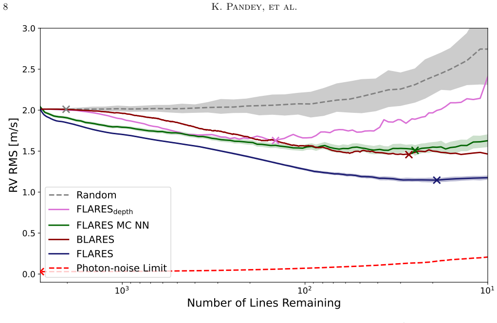
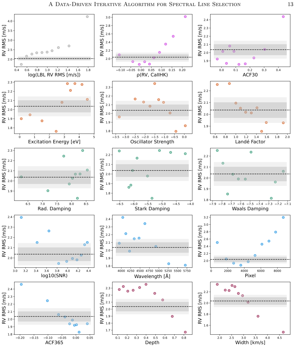
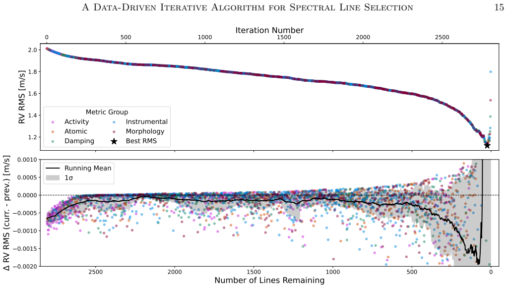
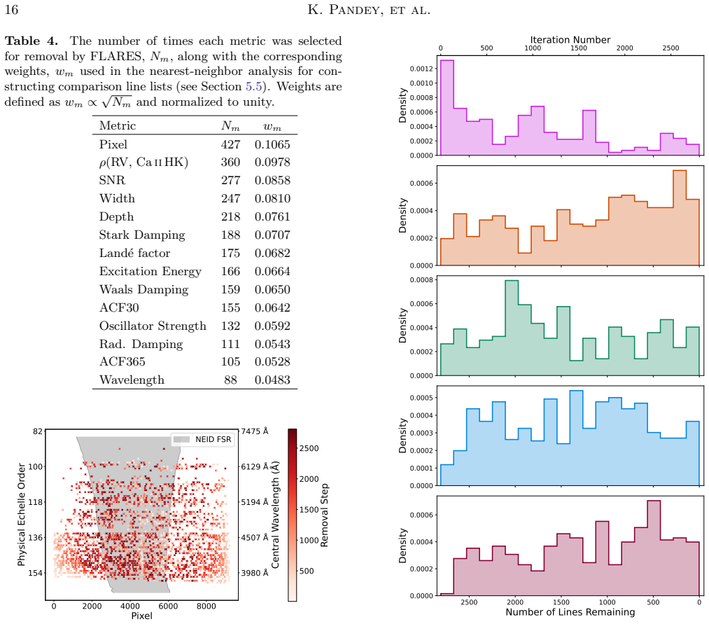
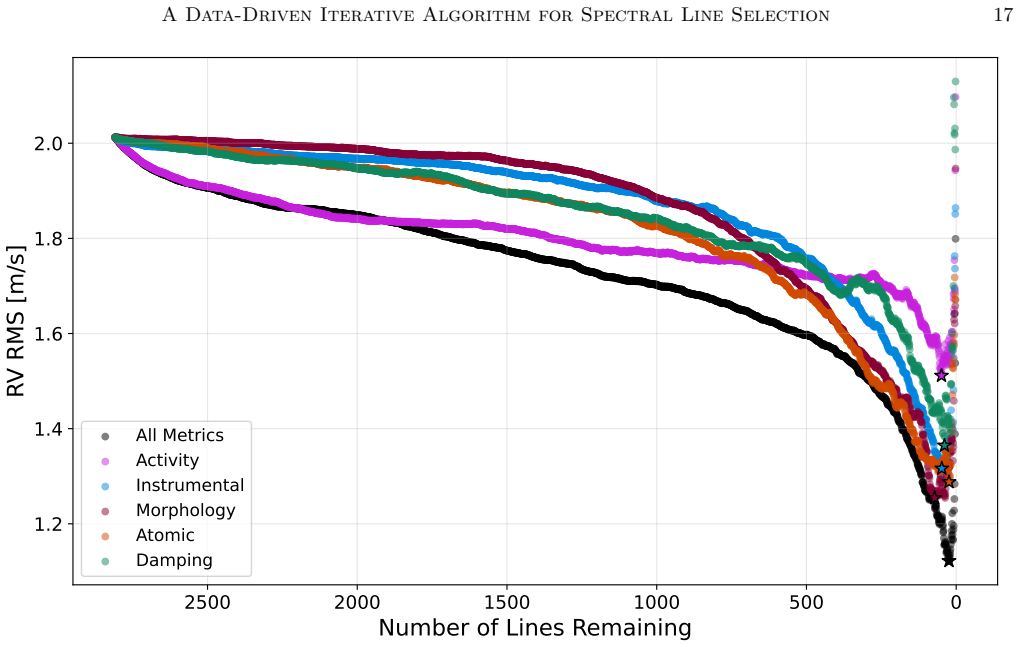
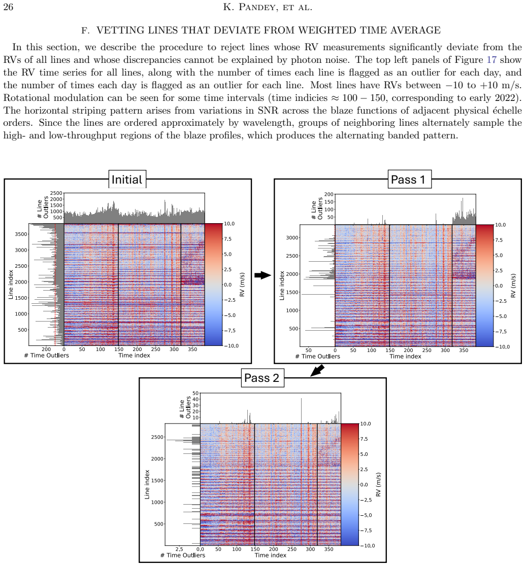
FLARES selects candidate spectral lines with extreme values of multiple line metrics such as depth, signal-to-noise ratio, and detector position, then iteratively rejects lines whose removal produces the largest decrease in weighted RV scatter. On 383 days of NEID solar observations this yields an RV RMS of 1.122 m/s with only 24 lines, which is lower than the 2.012 m/s obtained from the full line-by-line list and also lower than several benchmark selection methods. Monte Carlo tests confirm the selections are reproducible, and comparisons with alternative lists matched on similar properties show that FLARES is identifying the combination of line traits that actually drive the improvement.
What carries the argument
FLARES, an iterative line-selection algorithm that ranks and prunes lines using multiple metrics including depth, SNR, and position to minimize weighted RV scatter.
If this is right
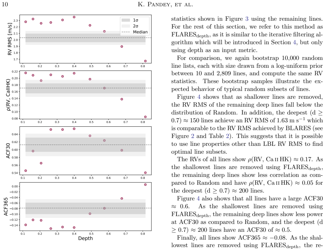
- Subsets chosen by line metrics such as depth and intrinsic RV scatter produce lower RV RMS than the full line list or random subsets of equal size.
- FLARES reaches 1.122 m/s RMS with 24 lines and outperforms the benchmark selection methods tested.
- Monte Carlo simulations show the FLARES selections are robust and reproducible.
- Alternative lists matched on similar properties to the FLARES lines do not achieve the same RV performance, confirming the algorithm identifies effective combinations of line traits.
Where Pith is reading between the lines
- If the solar-derived metrics transfer, FLARES could be run once on calibration data and then used on science targets without per-star adjustment.
- Focusing on a small number of lines may lower the computational cost of line-by-line analysis and reduce the influence of instrument artifacts that affect only certain detector regions.
- The same selection logic could be tested on data from other spectrographs to see whether the retained lines remain optimal across instruments.
Load-bearing premise
Line metrics and rejection rules derived from solar observations will identify similarly high-performing lines when applied to other stars without star-specific re-tuning.
What would settle it
Apply the FLARES line list derived from solar data to a different star and check whether its RV RMS remains lower than that of the full line list or random subsets of equal size on the same observations.
Figures


read the original abstract
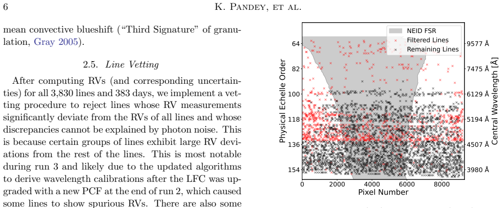
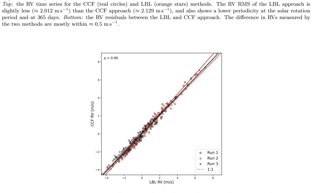
Independent analysis of individual spectral lines, or line-by-line (LBL) analyses, can improve upon standard cross-correlation function (CCF) methods for measuring radial velocities (RVs) because they preserve critical information about individual line shape changes that can be caused by stellar activity. In this work, we measure LBL RVs of 3,830 spectral lines across 383 days of NEID solar observations. Our LBL approach achieves an RV RMS of $2.012~\mathrm{m\,s^{-1}}$, which is slightly lower than the $2.129~\mathrm{m\,s^{-1}}$ achieved by a CCF approach using a shared line list. Then, we describe and benchmark several methods for selecting line lists based on line properties such as depth and intrinsic RV scatter. We find that these subsets have a lower RV RMS compared to either the full line list or random subsets of equal size. Motivated by these results, we present FLARES (Filtering Lines for Accurate Radial-velocity Exoplanet Search), an iterative line-selection algorithm. FLARES selects candidate spectral lines with extreme values of multiple line metrics and properties such as depth, signal-to-noise ratio, and detector position, and preferentially rejects lines whose removal produces the largest decrease in the weighted RV scatter. FLARES achieves an RV RMS of $1.122~\mathrm{m\,s^{-1}}$ using just 24 lines and performs better than the benchmark methods. We perform Monte Carlo simulations and show FLARES is robust and reproducible. Comparisons to alternative line lists chosen to have properties similar to the best FLARES-selected lines demonstrate that FLARES is successfully identifying line properties that lead to effective line lists for future extreme-precision RV measurements.
Editorial analysis
A structured set of objections, weighed in public.
Referee Report
Summary. The manuscript introduces FLARES, an iterative data-driven algorithm for selecting optimal spectral lines in line-by-line (LBL) radial velocity analysis. On 383 days of NEID solar observations measuring 3830 lines, the full LBL approach yields 2.012 m/s RMS (vs. 2.129 m/s for CCF), while FLARES selects 24 lines to reach 1.122 m/s RMS, outperforming random and property-matched subsets; Monte Carlo simulations are cited to show robustness and reproducibility.
Significance. If the selected line properties generalize, FLARES could meaningfully advance extreme-precision RV work by providing a reproducible method to minimize scatter from activity or instrumental effects. The concrete RMS values, direct comparisons to benchmarks, and use of a large homogeneous solar time series are strengths for internal validation on solar data.
major comments (3)
- [Abstract] Abstract: the claim that FLARES produces line lists 'suitable for future extreme-precision RV measurements' rests on an untested assumption that solar-derived metrics (depth, SNR, detector position, and iterative scatter thresholds) will identify high-performing lines on other stars; no independent stellar dataset or non-solar test is described.
- [FLARES algorithm] FLARES algorithm description: the target line count (24) and extreme-value thresholds for candidate selection are treated as fixed inputs without a sensitivity study or pre-specification, leaving open whether they were adjusted after inspecting the final RMS on the same 383-day series.
- [Evaluation] Evaluation and Monte Carlo section: the iterative rejection step uses weighted RV scatter computed from the identical time series that supplies the reported 1.122 m/s RMS; although Monte Carlo reproducibility checks are mentioned, no explicit cross-validation split or held-out solar subset is detailed to separate selection from evaluation.
minor comments (2)
- [Methods] Clarify whether the CCF comparison uses the identical line list or a standard mask, and report the exact weighting scheme applied to the RV scatter in the iterative step.
- [Abstract] The abstract states 'we perform Monte Carlo simulations and show FLARES is robust'; add a brief description of the simulation design (e.g., number of trials, what is randomized) to the main text.
Simulated Author's Rebuttal
We thank the referee for the detailed and constructive review. We address each major comment below, indicating where revisions will be made to strengthen the manuscript.
read point-by-point responses
-
Referee: [Abstract] Abstract: the claim that FLARES produces line lists 'suitable for future extreme-precision RV measurements' rests on an untested assumption that solar-derived metrics (depth, SNR, detector position, and iterative scatter thresholds) will identify high-performing lines on other stars; no independent stellar dataset or non-solar test is described.
Authors: Solar data from NEID provides the highest-SNR, most homogeneous time series available for isolating line-selection effects without stellar activity contamination. The metrics used (depth, SNR, detector position, scatter) are physical properties expected to generalize across targets observed with the same spectrograph. We agree, however, that the abstract claim is stronger than the solar-only validation supports. We will revise the abstract to describe the FLARES lines as 'promising candidates for' extreme-precision RV measurements and add a sentence noting that extension to stellar targets is planned future work. revision: partial
-
Referee: [FLARES algorithm] FLARES algorithm description: the target line count (24) and extreme-value thresholds for candidate selection are treated as fixed inputs without a sensitivity study or pre-specification, leaving open whether they were adjusted after inspecting the final RMS on the same 383-day series.
Authors: The target count of 24 was chosen to yield a compact list comparable in size to typical CCF line masks while still achieving substantial RMS reduction; the extreme-value thresholds were set to isolate clear outliers in the four line metrics. These choices were made prior to the final reported RMS. To remove any ambiguity, we will add a sensitivity analysis in the revised manuscript that varies both the target count (e.g., 10–50 lines) and the percentile thresholds, showing that the performance gain remains robust in the vicinity of the adopted values. revision: yes
-
Referee: [Evaluation] Evaluation and Monte Carlo section: the iterative rejection step uses weighted RV scatter computed from the identical time series that supplies the reported 1.122 m/s RMS; although Monte Carlo reproducibility checks are mentioned, no explicit cross-validation split or held-out solar subset is detailed to separate selection from evaluation.
Authors: The Monte Carlo procedure already draws random temporal subsets to test selection stability, but we acknowledge that it does not constitute a formal train/test split that fully decouples selection from evaluation. We will revise the Evaluation section to include an explicit k-fold cross-validation: line selection is performed on training folds only, the resulting line list is applied to the held-out fold, and the average out-of-sample RMS is reported. This will be added alongside the existing Monte Carlo results. revision: yes
Circularity Check
FLARES reported RMS is the direct output of iterative optimization on the identical solar time series used for evaluation
specific steps
-
fitted input called prediction
[Abstract]
"FLARES selects candidate spectral lines with extreme values of multiple line metrics and properties such as depth, signal-to-noise ratio, and detector position, and preferentially rejects lines whose removal produces the largest decrease in the weighted RV scatter. FLARES achieves an RV RMS of 1.122 m s^{-1} using just 24 lines and performs better than the benchmark methods."
The rejection step directly optimizes the weighted RV scatter computed from the 383-day solar series; the quoted 1.122 m/s RMS is the value of that same scatter after the optimization has been performed on the identical observations. No held-out partition or external stellar dataset is used for the final number.
full rationale
The paper derives line metrics and the iterative rejection rule from the 383-day NEID solar observations, then applies the rejection criterion (largest decrease in weighted RV scatter) to produce a 24-line list whose scatter is reported as 1.122 m/s. Because the selection explicitly minimizes the same scatter metric on the same dataset, the headline performance number is the fitted result rather than an independent test. Monte Carlo runs address only internal reproducibility within that sample. No self-citation chains, definitional loops, or imported uniqueness theorems appear; the circularity is confined to the fitted-input-called-prediction pattern in the evaluation step.
Axiom & Free-Parameter Ledger
free parameters (2)
- target line count (24)
- extreme-value thresholds for candidate selection
axioms (2)
- domain assumption Line depth, SNR, and detector position are predictive of a line's contribution to RV scatter.
- domain assumption Weighted RV scatter is a reliable scalar metric for line quality.
Reference graph
Works this paper leans on
-
[1]
Valenti, J. A. 2022, A&A, 664, A34, doi: 10.1051/0004-6361/202243276 Al Moulla, K., Dumusque, X., Figueira, P., et al. 2023, A&A, 669, A39, doi: 10.1051/0004-6361/202244663 Anglada-Escud´ e, G., & Tuomi, M. 2012, A&A, 548, A58, doi: 10.1051/0004-6361/201219910
-
[2]
1996, A&AS, 119, 373
Baranne, A., Queloz, D., Mayor, M., et al. 1996, A&AS, 119, 373
1996
-
[3]
2014, A&A, 564, A46, doi: 10.1051/0004-6361/201322383
Bodichon, R. 2014, A&A, 564, A46, doi: 10.1051/0004-6361/201322383
-
[4]
2011, A&A, 528, A4, doi: 10.1051/0004-6361/201014354
Boisse, I., Bouchy, F., H´ ebrard, G., et al. 2011, A&A, 528, A4, doi: 10.1051/0004-6361/201014354
-
[5]
2001, A&A, 374, 733, doi: 10.1051/0004-6361:20010730
Bouchy, F., Pepe, F., & Queloz, D. 2001, A&A, 374, 733, doi: 10.1051/0004-6361:20010730
-
[6]
A., Dumusque, X., & Halverson, S
Burt, J. A., Dumusque, X., & Halverson, S. 2025, arXiv e-prints, arXiv:2511.01954, doi: 10.48550/arXiv.2511.01954
-
[7]
Butler, R. P., Marcy, G. W., Williams, E., et al. 1996, PASP, 108, 500, doi: 10.1086/133755
-
[8]
1985, A&A, 150, 256
Cavallini, F., Ceppatelli, G., & Righini, A. 1985, A&A, 150, 256
1985
-
[9]
Christiansen, J. L., McElroy, D. L., Harbut, M., et al. 2025, PSJ, 6, 186, doi: 10.3847/PSJ/ade3c2 Collier Cameron, A., Mortier, A., Phillips, D., et al. 2019, MNRAS, 487, 1082, doi: 10.1093/mnras/stz1215
-
[10]
Ground-based and Airborne Instrumentation for Astronomy IV , year = 2012, editor =
Cosentino, R., Lovis, C., Pepe, F., et al. 2012, in Society of Photo-Optical Instrumentation Engineers (SPIE) Conference Series, Vol. 8446, Ground-based and Airborne Instrumentation for Astronomy IV, ed. I. S. McLean, S. K. Ramsay, & H. Takami, 84461V, doi: 10.1117/12.925738
-
[11]
Crass, J., Gaudi, B. S., Leifer, S., et al. 2021, arXiv e-prints, arXiv:2107.14291, doi: 10.48550/arXiv.2107.14291
-
[12]
2020, A&A, 633, A76, doi: 10.1051/0004-6361/201936548
Lovis, C. 2020, A&A, 633, A76, doi: 10.1051/0004-6361/201936548
-
[13]
Cretignier, M., Dumusque, X., Hara, N. C., & Pepe, F. 2021, A&A, 653, A43, doi: 10.1051/0004-6361/202140986
-
[14]
1982, ARA&A, 20, 61, doi: 10.1146/annurev.aa.20.090182.000425
Dravins, D. 1982, ARA&A, 20, 61, doi: 10.1146/annurev.aa.20.090182.000425
-
[15]
1981, A&A, 96, 345
Dravins, D., Lindegren, L., & Nordlund, A. 1981, A&A, 96, 345
1981
-
[16]
Dumusque, X. 2018, A&A, 620, A47, doi: 10.1051/0004-6361/201833795 30K. Pandey, et al
-
[17]
Dumusque, X., Boisse, I., & Santos, N. C. 2014, ApJ, 796, 132, doi: 10.1088/0004-637X/796/2/132
-
[18]
2011a, A&A, 527, A82, doi: 10.1051/0004-6361/201015877
Bonfils, X. 2011a, A&A, 527, A82, doi: 10.1051/0004-6361/201015877
-
[19]
Monteiro, M. J. P. F. G. 2011b, A&A, 525, A140, doi: 10.1051/0004-6361/201014097
-
[20]
2025, arXiv e-prints, arXiv:2510.27635, doi: 10.48550/arXiv.2510.27635
Dumusque, X., Al Moulla, K., Cretignier, M., et al. 2025, arXiv e-prints, arXiv:2510.27635, doi: 10.48550/arXiv.2510.27635
-
[21]
Edelson, R. A., & Krolik, J. H. 1988, ApJ, 333, 646, doi: 10.1086/166773
-
[22]
Ford, E. B., Bender, C. F., Blake, C. H., et al. 2024, arXiv e-prints, arXiv:2408.13318, doi: 10.48550/arXiv.2408.13318
-
[23]
R., Howard, A
Gibson, S. R., Howard, A. W., Rider, K., et al. 2024, in Society of Photo-Optical Instrumentation Engineers (SPIE) Conference Series, Vol. 13096, Ground-based and Airborne Instrumentation for Astronomy X, ed. J. J
2024
-
[24]
Bryant, K. Motohara, & J. R. D. Vernet, 1309609, doi: 10.1117/12.3017841
-
[25]
Gilbertson, C., Ford, E. B., Halverson, S., et al. 2024, arXiv e-prints, arXiv:2408.17289, doi: 10.48550/arXiv.2408.17289
-
[26]
Gray, D. F. 2005, The Observation and Analysis of Stellar Photospheres, doi: 10.1017/CBO9781316036570
-
[27]
2016, in Society of Photo-Optical Instrumentation Engineers (SPIE) Conference Series, Vol
Halverson, S., Terrien, R., Mahadevan, S., et al. 2016, in Society of Photo-Optical Instrumentation Engineers (SPIE) Conference Series, Vol. 9908, Ground-based and Airborne Instrumentation for Astronomy VI, ed. C. J
2016
-
[28]
Evans, L. Simard, & H. Takami, 99086P, doi: 10.1117/12.2232761
-
[29]
D., Collier Cameron, A., Unruh, Y
Haywood, R. D., Collier Cameron, A., Unruh, Y. C., et al. 2016, MNRAS, 457, 3637, doi: 10.1093/mnras/stw187
-
[30]
2020, arXiv e-prints, arXiv:2005.14083, doi: 10.48550/arXiv.2005.14083
Holzer, P., Cisewski-Kehe, J., Fischer, D., & Zhao, L. 2020, arXiv e-prints, arXiv:2005.14083, doi: 10.48550/arXiv.2005.14083
-
[31]
2016, in Society of Photo-Optical Instrumentation Engineers (SPIE) Conference Series, Vol
Jurgenson, C., Fischer, D., McCracken, T., et al. 2016, in Society of Photo-Optical Instrumentation Engineers (SPIE) Conference Series, Vol. 9908, Ground-based and Airborne Instrumentation for Astronomy VI, ed. C. J
2016
-
[32]
Evans, L. Simard, & H. Takami, 99086T, doi: 10.1117/12.2233002
-
[33]
Kjeldsen, H., & Bedding, T. R. 1995, A&A, 293, 87, doi: 10.48550/arXiv.astro-ph/9403015
work page internal anchor Pith review Pith/arXiv arXiv doi:10.48550/arxiv.astro-ph/9403015 1995
-
[34]
R., & Christensen-Dalsgaard, J
Kjeldsen, H., Bedding, T. R., & Christensen-Dalsgaard, J. 2008, ApJL, 683, L175, doi: 10.1086/591667
-
[35]
2021, A&A, 652, A28, doi: 10.1051/0004-6361/202140605
Lafarga, M., Ribas, I., Reiners, A., et al. 2021, A&A, 652, A28, doi: 10.1051/0004-6361/202140605
-
[36]
2010, A&A, 512, A38, doi: 10.1051/0004-6361/200913071
Lagrange, A.-M., Desort, M., & Meunier, N. 2010, A&A, 512, A38, doi: 10.1051/0004-6361/200913071
-
[37]
2011, A&A, 528, L9, doi: 10.1051/0004-6361/201016354
Lagrange, A.-M., Meunier, N., Desort, M., & Malbet, F. 2011, A&A, 528, L9, doi: 10.1051/0004-6361/201016354
-
[38]
Lakeland, B. S., Naylor, T., Haywood, R. D., et al. 2024, MNRAS, 527, 7681, doi: 10.1093/mnras/stad3723
-
[39]
F., Molaro, P., Monaco, L., & Haywood, R
Lanza, A. F., Molaro, P., Monaco, L., & Haywood, R. D. 2016, A&A, 587, A103, doi: 10.1051/0004-6361/201527379
-
[40]
Lin, A. S. J., Monson, A., Mahadevan, S., et al. 2022, AJ, 163, 184, doi: 10.3847/1538-3881/ac5622
-
[41]
Lovis, C., Dumusque, X., Santos, N. C., et al. 2011, arXiv e-prints, arXiv:1107.5325, doi: 10.48550/arXiv.1107.5325
work page internal anchor Pith review Pith/arXiv arXiv doi:10.48550/arxiv.1107.5325 2011
-
[42]
Luhn, J. K., Wright, J. T., Howard, A. W., & Isaacson, H. 2020, AJ, 159, 235, doi: 10.3847/1538-3881/ab855a
-
[43]
, year = 1995, month = nov, volume =
Mayor, M., & Queloz, D. 1995, Nature, 378, 355, doi: 10.1038/378355a0
-
[44]
McMillan, R. S., Moore, T. L., Perry, M. L., & Smith, P. H. 1993, ApJ, 403, 801, doi: 10.1086/172251
-
[45]
2010, A&A, 512, A39, doi: 10.1051/0004-6361/200913551
Meunier, N., Desort, M., & Lagrange, A.-M. 2010, A&A, 512, A39, doi: 10.1051/0004-6361/200913551
-
[46]
2015, A&A, 583, A118, doi: 10.1051/0004-6361/201525721
Meunier, N., Lagrange, A.-M., Borgniet, S., & Rieutord, M. 2015, A&A, 583, A118, doi: 10.1051/0004-6361/201525721
-
[47]
2017, A&A, 607, A124, doi: 10.1051/0004-6361/201731017 O’Sullivan, N
Meunier, N., Mignon, L., & Lagrange, A.-M. 2017, A&A, 607, A124, doi: 10.1051/0004-6361/201731017 O’Sullivan, N. K., Aigrain, S., Cretignier, M., et al. 2025, MNRAS, 541, 3942, doi: 10.1093/mnras/staf1168
-
[48]
Palumbo, M. L., Ford, E. B., Gonzalez, E. B., et al. 2024, AJ, 168, 46, doi: 10.3847/1538-3881/ad4c6d
-
[49]
2026, Supplementary Material for Improving the Precision of Line-by-Line Radial Velocities: A Data-Driven Iterative Algorithm for Spectral Line
Pandey, K. 2026, Supplementary Material for Improving the Precision of Line-by-Line Radial Velocities: A Data-Driven Iterative Algorithm for Spectral Line
2026
-
[50]
Selection, Zenodo, doi: 10.5281/zenodo.20937741
-
[51]
Pepe, F., Mayor, M., Galland, F., et al. 2002, A&A, 388, 632, doi: 10.1051/0004-6361:20020433
-
[52]
2004, A&A, 423, 385, doi: 10.1051/0004-6361:20040389
Pepe, F., Mayor, M., Queloz, D., et al. 2004, A&A, 423, 385, doi: 10.1051/0004-6361:20040389
-
[53]
2013, The Messenger, 153, 6
Pepe, F., Cristiani, S., Rebolo, R., et al. 2013, The Messenger, 153, 6
2013
-
[54]
Ryabchikova, T., Piskunov, N., Kurucz, R. L., et al. 2015, PhyS, 90, 054005, doi: 10.1088/0031-8949/90/5/054005
-
[55]
Saar, S. H. 2003, in Astronomical Society of the Pacific Conference Series, Vol. 294, Scientific Frontiers in Research on Extrasolar Planets, ed. D. Deming & S. Seager, 65–70
2003
-
[56]
Saar, S. H., & Donahue, R. A. 1997, ApJ, 485, 319, doi: 10.1086/304392
-
[57]
Salzer, J., Cisewski-Kehe, J., Ford, E. B., & Zhao, L. L. 2025, AJ, 170, 179, doi: 10.3847/1538-3881/adf29d A Data-Driven Iterative Algorithm for Spectral Line Selection31
-
[58]
2016, in Society of Photo-Optical Instrumentation Engineers (SPIE) Conference Series, Vol
Schwab, C., Rakich, A., Gong, Q., et al. 2016, in Society of Photo-Optical Instrumentation Engineers (SPIE) Conference Series, Vol. 9908, Ground-based and Airborne Instrumentation for Astronomy VI, ed. C. J. Evans, L. Simard, & H. Takami, 99087H, doi: 10.1117/12.2234411
-
[59]
L., & Schwab, C
Seifahrt, A., St¨ urmer, J., Bean, J. L., & Schwab, C. 2018, in Society of Photo-Optical Instrumentation Engineers (SPIE) Conference Series, Vol. 10702, Ground-based and Airborne Instrumentation for Astronomy VII, ed. C. J
2018
-
[60]
Evans, L. Simard, & H. Takami, 107026D, doi: 10.1117/12.2312936
-
[61]
Winn, J. N., & Fabrycky, D. C. 2015, ARA&A, 53, 409, doi: 10.1146/annurev-astro-082214-122246
-
[62]
Wright, J. T., & Kanodia, S. 2020, PSJ, 1, 38, doi: 10.3847/PSJ/ababa4
-
[63]
Zechmeister, M., Reiners, A., Amado, P. J., et al. 2018, A&A, 609, A12, doi: 10.1051/0004-6361/201731483
-
[64]
Zhao, L. L., Dumusque, X., Ford, E. B., et al. 2023, AJ, 166, 173, doi: 10.3847/1538-3881/acf83e
discussion (0)
Sign in with ORCID, Apple, or X to comment. Anyone can read and Pith papers without signing in.