Higher-order time-stepping schemes for fluid-structure interaction problems
Pith reviewed 2026-05-25 12:29 UTC · model grok-4.3
The pith
Second-order BDF and Crank-Nicolson schemes are stable for distributed Lagrange multiplier fluid-structure interaction formulations.
A machine-rendered reading of the paper's core claim, the machinery that carries it, and where it could break.
Core claim
The authors establish that the recently introduced distributed Lagrange multiplier formulation for fluid-structure interaction remains stable under second-order backward differentiation formulae and Crank-Nicolson time integration, with the stability properties shown theoretically and verified through numerical experiments that match the analysis.
What carries the argument
The distributed Lagrange multiplier formulation for fluid-structure interaction, extended by second-order BDF and Crank-Nicolson time-stepping schemes.
If this is right
- Higher temporal accuracy becomes available for long-time FSI simulations without sacrificing stability.
- The fictitious-domain treatment of the fluid-structure interface continues to function under the higher-order integrators.
- The theoretical stability results provide a basis for reliable error control in coupled problems.
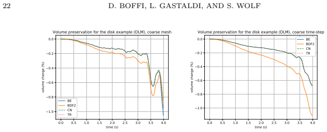
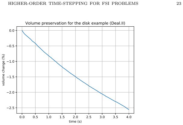
- Numerical confirmation shows the methods perform as predicted on standard test cases.
Where Pith is reading between the lines
- The same stability framework could be tested on related multiphysics couplings that use distributed multipliers.
- Implementation in existing finite-element libraries would allow direct comparison of first- and second-order time accuracy on the same spatial mesh.
- Extension to variable-step or adaptive BDF variants might preserve the stability property if the multiplier constraint is handled consistently.
Load-bearing premise
The distributed Lagrange multiplier formulation for fluid-structure interaction stays well-posed and compatible with the chosen second-order time integrators under the given spatial discretization.
What would settle it
A concrete FSI benchmark computation in which the combined scheme produces growing oscillations or violates a discrete energy estimate would falsify the stability claim.
Figures

read the original abstract
We consider a recently introduced formulation for fluid-structure interaction problems which makes use of a distributed Lagrange multiplier in the spirit of the fictitious domain method. In this paper we focus on time integration methods of second order based on backward differentiation formulae and on the Crank-Nicolson method. We show the stability properties of the resulting method; numerical tests confirm the theoretical results.
Editorial analysis
A structured set of objections, weighed in public.
Referee Report
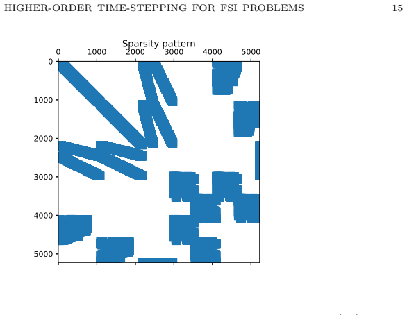
Summary. The manuscript develops second-order time integration schemes (BDF2 and Crank-Nicolson) for fluid-structure interaction problems discretized via a distributed Lagrange multiplier fictitious-domain formulation. It derives stability via energy estimates that extend from the continuous problem to the fully discrete scheme under standard inf-sup assumptions on the spatial elements, and verifies the predicted stability and convergence rates through numerical experiments.
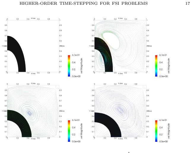
Significance. The central contribution is a stability result for higher-order time integrators in a DLM-FSI setting, supported by an energy identity that carries over without post-hoc fitting. This is a concrete advance for long-time FSI simulations where first-order schemes are often used for stability reasons. The numerical tests are consistent with the analysis and provide evidence that the discrete coupling terms do not destroy the energy balance.
minor comments (3)
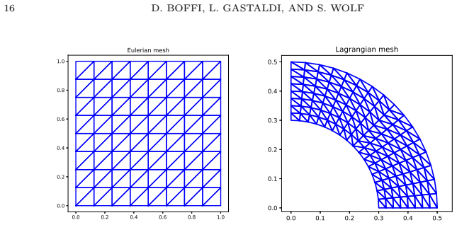
- [§3] The description of the spatial discretization (inf-sup stable elements and quadrature rules) in §3 could be made more explicit by stating the precise finite-element spaces and the quadrature order used for the multiplier terms, as this is load-bearing for the discrete energy estimate.
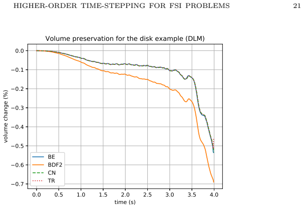
- Figure 4 (or the corresponding convergence plot) would benefit from error bars or multiple mesh sizes to illustrate that the observed rates are robust rather than single-run artifacts.
- [§4] A short remark on how the initial data for the second-order schemes are obtained (e.g., via a first-order step or extrapolation) would clarify the start-up procedure and avoid ambiguity in the stability proof.
Simulated Author's Rebuttal
We thank the referee for the careful reading and positive assessment of our manuscript, including the accurate summary of the stability analysis for the BDF2 and Crank-Nicolson schemes in the DLM-FSI setting and the recommendation for minor revision. No specific major comments were listed in the report.
Circularity Check
No significant circularity
full rationale
The derivation chain consists of an energy estimate for the continuous DLM-FSI problem that is shown to carry over to the fully discrete scheme for BDF2 and Crank-Nicolson under standard inf-sup and quadrature assumptions on the spatial discretization. This is a direct stability proof, not a re-derivation of fitted quantities or a renaming of prior results. The 'recently introduced' DLM formulation is taken as an external premise whose well-posedness is addressed in the analysis rather than presupposed by self-citation alone. No equation reduces to its own inputs by construction, and no load-bearing uniqueness claim is imported from overlapping-author prior work.
Axiom & Free-Parameter Ledger
Reference graph
Works this paper leans on
-
[1]
D. Boffi, N. Cavallini, F. Gardini, and L. Gastaldi. Local Mass Conservation of Stokes Finite Elements. J. Sci. Comput. , 52:383400, 2012
work page 2012
-
[2]
D. Boffi, N. Cavallini, and L. Gastaldi. Finite Element approach to Immersed Bound- ary Method with different fluid and solid densities. Math. Models Methods Appl. Sci , 21(12):25232550, 2011
work page 2011
-
[3]
D. Boffi, N. Cavallini, and L. Gastaldi. The Finite Element Immersed Boundary Method with Distributed Lagrange Multiplier. SIAM J. Numer. Anal. , 53(6):2584–2604, 2015
work page 2015
- [4]
- [5]
-
[6]
D. Boffi, L. Gastaldi, and L. Heltai. Numerical stability of The Finite Element Immersed Boundary Method. Mathematical Models and Methods in Applied Sciences , 17:14791505, 2007
work page 2007
-
[7]
D. Boffi, L. Gastaldi, and L. Heltai. A distributed Lagrange formulation of the Finite El- ement Immersed Boundary Method for fluids interacting with compressible solids. In Boffi D., Pavarino L., Rozza G., Scacchi S., and Vergara C., editors, Mathematical and Numer- ical Modeling of the Cardiovascular System and Applications , volume 16 of SEMA SIMAI Springer...
work page 2018
-
[8]
D. Boffi, L. Gastaldi, L. Heltai, and C. S. Peskin. On the hyper-elastic formulation of the immersed boundary method. Comput. Methods Appl. Mech. Eng. , 197:22102231, 2008
work page 2008
-
[9]
W. Chen, M. Gunzburger, D. Sun, and X. Wang. Efficient and long-time accurate second- order methods for Stokes-Darcy Systems. SIAM J. Numer. Anal. , 51(5):2563–2584, 2013
work page 2013
-
[10]
Peter Deuflhard and Folkmar Bornemann. Numerische Mathematik 2 . de Gruyter Lehrbuch. [de Gruyter Textbook]. Walter de Gruyter & Co., Berlin, revised edition, 2008. Gew¨ ohnliche Differentialgleichungen. [Ordinary differential equations]
work page 2008
-
[11]
S. Dong. BDF-like methods for nonlinear dynamic analysis. J. Comput. Phys., 229:30193045, 2010
work page 2010
-
[12]
B. E. Griffith. On the Volume Conservation of the Immersed Boundary Method. Commun. Comput. Phys., 12(02):401432, 2012
work page 2012
-
[13]
B. E. Griffith and X. Luo. Hybrid finite difference/finite element immersed boundary method. Int. J. Numer. Meth. Biomed. Engng. , 33(12):e2888, 2012. 24 D. BOFFI, L. GASTALDI, AND S. WOLF
work page 2012
-
[14]
L. Heltai and F. Costanzo. Variational Implementation of Immersed Finite Element Methods. Comput. Methods Appl. Mech. Eng. , 229-232:110 – 127, 2012
work page 2012
-
[15]
J. Heywood and R. Rannacher. Finite-Element Approximation of the Nonstationary Navier- Stokes Problem. Part IV: Error Analysis for Second-Order Time Discretization. SIAM J. Numer. Anal., 27(2):353–384, 1990
work page 1990
-
[16]
O. R. Isik, G. Yuksel, and B. Demir. Analysis of second order and unconditionally stable BDF2-AB2 method for the Navier-Stokes equations with nonlinear time relaxation. Numer. Methods Partial Differ. Equations , 34(6):2060–2078, 2017
work page 2060
-
[17]
V. John. Finite Element Methods for Incompressible Flow Problems . Springer, 2016
work page 2016
-
[18]
Y. Okamoto, K. Fujiwara, and Y. Ishihara. Effectiveness of Higher Order Time Integration in Time-Domain Finite-Element Analysis. IEEE Transactions on Magnetics, 46(8):3321 – 3324, Aug 2010
work page 2010
-
[19]
C. S. Peskin. The immersed boundary method. Acta Numerica, 11:479517, 2002
work page 2002
-
[20]
S. Roy, L. Heltai, and F. Costanzo. Benchmarking the Immersed Finite Element Method for Fluid-Structure Interaction Problems. Comput. Math. Appl. , 69(10):1167 – 1188, 2015
work page 2015
-
[21]
X. Wang and L. T. Zhang. Interpolation functions in the immersed boundary and finite element methods. Comput. Mech., 45(4):321, Dec 2009. E-mail address: daniele.boffi@unipv.it E-mail address: lucia.gastaldi@unibs.it E-mail address: s.wolf@tum.de
work page 2009
discussion (0)
Sign in with ORCID, Apple, or X to comment. Anyone can read and Pith papers without signing in.