Switchable Normalization for Learning-to-Normalize Deep Representation
Pith reviewed 2026-05-24 18:02 UTC · model grok-4.3
The pith
Switchable Normalization lets each layer learn to weight among channel, layer, and minibatch statistics.
A machine-rendered reading of the paper's core claim, the machinery that carries it, and where it could break.
Core claim
Switchable Normalization (SN) learns a set of importance weights for each normalization layer so that the layer can automatically select or blend among three distinct scopes for computing normalization statistics: channel-wise, layer-wise, and minibatch-wise. The weights are optimized jointly with the rest of the network parameters, allowing the choice of normalizer to adapt to network architecture, task, and data distribution without manual intervention or sensitive hyperparameters.
What carries the argument
The end-to-end learned importance weights that switch or combine channel normalization, layer normalization, and minibatch normalization for each individual layer.
If this is right
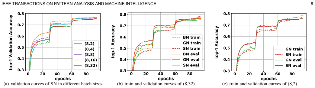
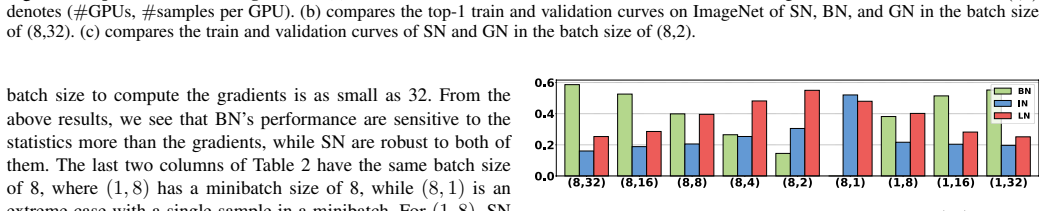
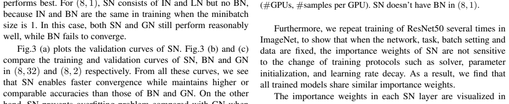
- SN maintains accuracy when minibatch size drops to two images per GPU, unlike standard batch normalization.
- SN removes the need to search over the number of groups required by group normalization.
- Different layers inside the same network can and do converge to different preferred normalizers.
- SN yields higher accuracy than any single fixed normalizer on ImageNet, COCO, Cityscapes, ADE20K, MegaFace, and Kinetics without architecture-specific changes.
Where Pith is reading between the lines
- The results imply that the best normalization scope is often position-dependent within a network rather than uniform across all layers.
- The same switching mechanism could be applied to additional normalization variants or to statistics computed over other dimensions such as spatial regions.
- In new domains with unusual batch sizes or data statistics, the learned weights might serve as a diagnostic for which normalizer properties matter most.
- One could measure whether the final importance weights correlate with network depth or with properties of the input distribution.
Load-bearing premise
End-to-end optimization of the importance weights will discover an effective per-layer selection rather than collapsing to an average or overfitting the training distribution.
What would settle it
Train an identical architecture with SN and with a single fixed normalizer on ImageNet; if the fixed version matches or exceeds SN accuracy while using the same batch size and training schedule, the benefit of the learned switch is not supported.
Figures




read the original abstract
We address a learning-to-normalize problem by proposing Switchable Normalization (SN), which learns to select different normalizers for different normalization layers of a deep neural network. SN employs three distinct scopes to compute statistics (means and variances) including a channel, a layer, and a minibatch. SN switches between them by learning their importance weights in an end-to-end manner. It has several good properties. First, it adapts to various network architectures and tasks. Second, it is robust to a wide range of batch sizes, maintaining high performance even when small minibatch is presented (e.g. 2 images/GPU). Third, SN does not have sensitive hyper-parameter, unlike group normalization that searches the number of groups as a hyper-parameter. Without bells and whistles, SN outperforms its counterparts on various challenging benchmarks, such as ImageNet, COCO, CityScapes, ADE20K, MegaFace, and Kinetics. Analyses of SN are also presented to answer the following three questions: (a) Is it useful to allow each normalization layer to select its own normalizer? (b) What impacts the choices of normalizers? (c) Do different tasks and datasets prefer different normalizers? We hope SN will help ease the usage and understand the normalization techniques in deep learning. The code of SN has been released at https://github.com/switchablenorms.
Editorial analysis
A structured set of objections, weighed in public.
Referee Report
Summary. The manuscript proposes Switchable Normalization (SN), which learns per-layer importance weights to select among three normalization scopes (channel/instance, layer, and minibatch) in an end-to-end fashion. The central claims are that SN adapts automatically to architectures and tasks, remains robust even at very small batch sizes (e.g., 2 images/GPU), requires no sensitive hyperparameters, and outperforms standard BN/IN/LN baselines on ImageNet, COCO, CityScapes, ADE20K, MegaFace, and Kinetics. The authors also present analyses addressing (a) whether per-layer selection is useful, (b) what influences normalizer choice, and (c) whether tasks/datasets prefer different normalizers. Public code release is noted.
Significance. If the empirical results and analyses hold, SN would be a practically useful contribution by removing the need to manually choose or tune normalization methods while delivering measurable gains across detection, segmentation, recognition, and video tasks. The released code is a clear strength for reproducibility. The three targeted analyses directly engage the question of whether learned switchability adds value beyond a fixed mixture, which mitigates the primary stress-test concern.
major comments (1)
- [§5] §5 (Analyses): the paper reports learned weight distributions and per-layer selections that are visibly non-uniform across layers and tasks; this directly addresses the possibility that optimization collapses to uniform averaging. No further control experiment against a fixed (1/3,1/3,1/3) mixture is required for the central claim once these distributions are shown.
minor comments (2)
- [Table 1, Figure 3] Table 1 and Figure 3: axis labels and legend entries for the three scopes should be standardized to the same terminology used in §3 (e.g., “IN”, “LN”, “BN”) to avoid reader confusion.
- [§4.2] §4.2: the statement that SN “does not have sensitive hyper-parameter” should be qualified by noting that the three-scope formulation itself is a modeling choice; a brief sentence acknowledging this would improve precision.
Simulated Author's Rebuttal
We thank the referee for the positive review and recommendation for minor revision. We address the single major comment below.
read point-by-point responses
-
Referee: [§5] §5 (Analyses): the paper reports learned weight distributions and per-layer selections that are visibly non-uniform across layers and tasks; this directly addresses the possibility that optimization collapses to uniform averaging. No further control experiment against a fixed (1/3,1/3,1/3) mixture is required for the central claim once these distributions are shown.
Authors: We appreciate the referee's assessment that the analyses in Section 5 are sufficient. The reported non-uniform weight distributions and per-layer selections across architectures and tasks demonstrate that SN does not collapse to uniform averaging, thereby supporting the value of learned switchability without requiring an additional fixed-mixture control experiment. revision: no
Circularity Check
No significant circularity in SN derivation or claims
full rationale
The paper defines Switchable Normalization via end-to-end learned importance weights over three normalization scopes (channel, layer, minibatch). Performance claims on ImageNet, COCO and other benchmarks are presented as empirical outcomes of this optimization, not as quantities forced equal to the inputs by any equation or self-citation chain. No load-bearing step reduces a prediction to a fitted constant, renames a known result, or imports uniqueness from prior author work. The method remains self-contained against external benchmarks; the reader's assessment of minor non-load-bearing self-citation aligns with a score of 0 here.
Axiom & Free-Parameter Ledger
axioms (1)
- domain assumption Normalization layers improve training stability and generalization in deep neural networks
Reference graph
Works this paper leans on
-
[1]
Batch normalization: Accelerating deep net- work training by reducing internal covariate shift,
S. Ioffe and C. Szegedy, “Batch normalization: Accelerating deep net- work training by reducing internal covariate shift,” in ICML, 2015
work page 2015
-
[2]
Instance Normalization: The Missing Ingredient for Fast Stylization
D. Ulyanov, A. Vedaldi, and V . Lempitsky, “Instance normalization: The missing ingredient for fast stylization,” arXiv:1607.08022, 2016
work page internal anchor Pith review Pith/arXiv arXiv 2016
-
[3]
J. L. Ba, J. R. Kiros, and G. E. Hinton, “Layer normalization,” arXiv:1607.06450, 2016
work page internal anchor Pith review Pith/arXiv arXiv 2016
-
[4]
Perceptual losses for real-time style transfer and super-resolution,
J. Johnson, A. Alahi, and L. Fei-Fei, “Perceptual losses for real-time style transfer and super-resolution,” in ECCV, 2016
work page 2016
- [5]
-
[6]
Deep residual learning for image recognition,
K. He, X. Zhang, S. Ren, and J. Sun, “Deep residual learning for image recognition,” in CVPR, 2016
work page 2016
-
[7]
Imagenet: A large-scale hierarchical image database,
J. Deng, W. Dong, R. Socher, L.-J. Li, K. Li, and L. Fei-Fei, “Imagenet: A large-scale hierarchical image database,” in CVPR, 2009
work page 2009
-
[8]
Imagenet large scale visual recognition challenge,
O. Russakovsky, J. Deng, H. Su, J. Krause, S. Satheesh, S. Ma, Z. Huang, A. Karpathy, A. Khosla, M. Bernstein et al., “Imagenet large scale visual recognition challenge,” International Journal of Computer Vision , vol. 115, no. 3, pp. 211–252, 2015
work page 2015
-
[9]
Microsoft coco: Common objects in context,
T.-Y . Lin, M. Maire, S. Belongie, J. Hays, P. Perona, D. Ramanan, P. Doll ´ar, and C. L. Zitnick, “Microsoft coco: Common objects in context,” in ECCV, 2014
work page 2014
-
[10]
The cityscapes dataset for semantic urban scene understanding,
M. Cordts, M. Omran, S. Ramos, T. Rehfeld, M. Enzweiler, R. Benenson, U. Franke, S. Roth, and B. Schiele, “The cityscapes dataset for semantic urban scene understanding,” in CVPR, 2016
work page 2016
-
[11]
Scene parsing through ADE20K dataset,
B. Zhou, H. Zhao, X. Puig, S. Fidler, A. Barriuso, and A. Torralba, “Scene parsing through ADE20K dataset,” in CVPR, 2017
work page 2017
-
[12]
The megaface benchmark: 1 million faces for recognition at scale,
I. Kemelmacher-Shlizerman, S. M. Seitz, D. Miller, and E. Brossard, “The megaface benchmark: 1 million faces for recognition at scale,” in CVPR, 2016
work page 2016
-
[13]
The Kinetics Human Action Video Dataset
W. Kay, J. Carreira, K. Simonyan, B. Zhang, C. Hillier, S. Vijaya- narasimhan, F. Viola, T. Green, T. Back, P. Natsev et al. , “The kinetics human action video dataset,” arXiv:1705.06950, 2017
work page internal anchor Pith review Pith/arXiv arXiv 2017
-
[14]
Efficient Neural Architecture Search via Parameter Sharing
H. Pham, M. Y . Guan, B. Zoph, Q. V . Le, and J. Dean, “Efficient neural architecture search via parameter sharing,” arXiv:1802.03268, 2018
work page internal anchor Pith review Pith/arXiv arXiv 2018
-
[15]
Batch renormalization: Towards reducing minibatch depen- dence in batch-normalized models,
S. Ioffe, “Batch renormalization: Towards reducing minibatch depen- dence in batch-normalized models,” in NIPS, 2017
work page 2017
-
[16]
Batch kalman nor- malization: Towards training deep neural networks with micro-batches,
G. Wang, J. Peng, P. Luo, X. Wang, and L. Lin, “Batch kalman nor- malization: Towards training deep neural networks with micro-batches,” NIPS, 2018
work page 2018
-
[17]
Weight normalization: A simple repa- rameterization to accelerate training of deep neural networks,
T. Salimans and D. P. Kingma, “Weight normalization: A simple repa- rameterization to accelerate training of deep neural networks,” in NIPS, 2016
work page 2016
-
[18]
Spectral normal- ization for generative adversarial networks,
T. Miyato, T. Kataoka, M. Koyama, and Y . Yoshida, “Spectral normal- ization for generative adversarial networks,” in ICLR, 2018
work page 2018
-
[19]
G. Desjardins, K. Simonyan, R. Pascanu, and K. Kavukcuoglu, “Natural neural networks,” NIPS, 2015
work page 2015
-
[20]
Learning deep architectures via generalized whitened neural networks,
P. Luo, “Learning deep architectures via generalized whitened neural networks,” ICML, 2017
work page 2017
-
[21]
S.-i. Amari and H. Nagaoka, Methods of information geometry . Amer- ican Mathematical Soc., 2007, vol. 191
work page 2007
-
[22]
The Shattered Gradients Problem: If resnets are the answer, then what is the question?
D. Balduzzi, M. Frean, L. Leary, J. Lewis, K. W.-D. Ma, and B. McWilliams, “The shattered gradients problem: If resnets are the answer, then what is the question?” arXiv preprint arXiv:1702.08591 , 2017
work page internal anchor Pith review Pith/arXiv arXiv 2017
-
[23]
How does batch normalization help optimization?(no, it is not about internal covariate shift),
S. Santurkar, D. Tsipras, A. Ilyas, and A. Madry, “How does batch normalization help optimization?(no, it is not about internal covariate shift),” in NIPS, 2018
work page 2018
-
[24]
Norm matters: efficient and accurate normalization schemes in deep networks,
E. Hoffer, R. Banner, I. Golan, and D. Soudry, “Norm matters: efficient and accurate normalization schemes in deep networks,” in NIPS, 2018
work page 2018
-
[25]
Towards understanding regularization in batch normalization,
P. Luo, X. Wang, W. Shao, and Z. Peng, “Towards understanding regularization in batch normalization,” ICLR, 2019
work page 2019
-
[26]
A mean field theory of batch normalization,
V . R. J. S.-D. S. S. S. Greg Yang, Jeffrey Pennington, “A mean field theory of batch normalization,” in ICLR, 2019
work page 2019
-
[27]
Theoretical analysis of auto rate- tuning by batch normalization,
K. L. Sanjeev Arora, Zhiyuan Li, “Theoretical analysis of auto rate- tuning by batch normalization,” in ICLR, 2019
work page 2019
-
[28]
Understanding batch normalization,
B. S. K. Q. W. Johan Bjorck, Carla Gomes, “Understanding batch normalization,” in NIPS, 2018
work page 2018
-
[29]
Normal- izing the normalizers: Comparing and extending network normalization schemes,
M. Ren, R. Liao, R. Urtasun, F. H. Sinz, and R. S. Zemel, “Normal- izing the normalizers: Comparing and extending network normalization schemes,” in ICLR, 2016. IEEE TRANSACTIONS ON PATTERN ANAL YSIS AND MACHINE INTELLIGENCE 16
work page 2016
-
[30]
Two at once: enhancing learning and generalization capacities via ibn-net,
J. S. Xinggang Pan, Ping Luo and X. Tang, “Two at once: enhancing learning and generalization capacities via ibn-net,” in ECCV, 2018
work page 2018
-
[31]
Differentiable dynamic normalization for learning deep representation,
P. Luo, P. Zhanglin, S. Wenqi, Z. Ruimao, R. Jiamin, and W. Lingyun, “Differentiable dynamic normalization for learning deep representation,” in ICML, 2019
work page 2019
-
[32]
Q. Liao, K. Kawaguchi, and T. Poggio, “Streaming normalization: To- wards simpler and more biologically-plausible normalizations for online and recurrent learning,” arXiv preprint arXiv:1610.06160, 2016
work page internal anchor Pith review Pith/arXiv arXiv 2016
-
[33]
Decorrelated batch normal- ization,
L. Huang, D. Yang, B. Lang, and J. Deng, “Decorrelated batch normal- ization,” in CVPR, 2018
work page 2018
-
[34]
Learning Visual Reasoning Without Strong Priors
E. Perez, H. de Vries, and F. Strub, “Learning visual reasoning without strong priors,” in arXiv:1707.03017, 2017
work page internal anchor Pith review Pith/arXiv arXiv 2017
-
[35]
Switchable whitening for deep representation learning,
X. Pan, X. Zhan, J. Shi, X. Tang, and P. Luo, “Switchable whitening for deep representation learning,” arXiv, 2019
work page 2019
-
[36]
Centered weight normalization in accelerating training of deep neural networks,
L. Huang, X. Liu, Y . Liu, B. Lang, and D. Tao, “Centered weight normalization in accelerating training of deep neural networks,” inICCV, 2017
work page 2017
-
[37]
I. J. Goodfellow, J. Pouget-Abadie, M. Mirza, B. Xu, D. Warde-Farley, S. Ozair, A. C. Courville, and Y . Bengio, “Generative adversarial nets,” in NIPS, 2014
work page 2014
-
[38]
Eigennet: Towards fast and structural learning of deep neural networks,
P. Luo, “Eigennet: Towards fast and structural learning of deep neural networks,” IJCAI, 2017
work page 2017
-
[39]
An overview of bilevel optimiza- tion,
B. Colson, P. Marcotte, and G. Savard, “An overview of bilevel optimiza- tion,” Annals of operations research , 2007
work page 2007
-
[40]
Gradient-based hyperpa- rameter optimization through reversible learning,
D. Maclaurin, D. Duvenaud, and R. Adams, “Gradient-based hyperpa- rameter optimization through reversible learning,” ICML, 2015
work page 2015
-
[41]
DARTS: Differentiable Architecture Search
H. Liu, K. Simonyan, and Y . Yang, “Darts: Differentiable architecture search,” arXiv:1806.09055, 2018
work page internal anchor Pith review Pith/arXiv arXiv 2018
-
[42]
Arbitrary style transfer in real-time with adaptive instance normalization,
X. Huang and S. Belongie, “Arbitrary style transfer in real-time with adaptive instance normalization,” in ICCV, 2017
work page 2017
-
[43]
D. Ulyanov, A. Vedaldi, and V . Lempitsky, “Improved texture networks: Maximizing quality and diversity in feed-forward stylization and texture synthesis,” in CVPR, 2017
work page 2017
-
[44]
Imagenet classification with deep convolutional neural networks,
A. Krizhevsky, I. Sutskever, and G. E. Hinton, “Imagenet classification with deep convolutional neural networks,” in NIPS, 2012
work page 2012
-
[45]
Accurate, Large Minibatch SGD: Training ImageNet in 1 Hour
P. Goyal, P. Dollr, R. Girshick, P. Noordhuis, L. Wesolowski, A. Kyrola, A. Tulloch, Y . Jia, and K. He, “Accurate, large minibatch sgd: Training imagenet in 1 hour,” arXiv:1706.02677, 2017
work page internal anchor Pith review Pith/arXiv arXiv 2017
-
[46]
Ssn: Learning sparse switchable normalization via sparsestmax,
W. Shao, T. Meng, J. Li, R. Zhang, Y . Li, X. Wang, and P. Luo, “Ssn: Learning sparse switchable normalization via sparsestmax,” in CVPR, 2019
work page 2019
-
[47]
Faster r-cnn: Towards real-time object detection with region proposal networks,
S. Ren, K. He, R. Girshick, and J. Sun, “Faster r-cnn: Towards real-time object detection with region proposal networks,” in NIPS, 2015
work page 2015
-
[48]
Feature Pyramid Networks for Object Detection
T.-Y . Lin, P. Dollra, R. Girshick, K. He, B. Hariharan, and S. Belongie, “Feature pyramid networks for object detection,” arXiv:1612.03144, 2016
work page internal anchor Pith review Pith/arXiv arXiv 2016
- [49]
-
[50]
R. Girshick, I. Radosavovic, G. Gkioxari, P. Doll ´ar, and K. He, “Detec- tron,” https:// github.com/ facebookresearch/ detectron, 2018
work page 2018
-
[51]
A faster pytorch implementation of faster r-cnn,
J. Yang, J. Lu, D. Batra, and D. Parikh, “A faster pytorch implementation of faster r-cnn,” https:// github.com/ jwyang/ faster-rcnn.pytorch, 2017
work page 2017
-
[52]
Megdet: A large mini-batch object detector,
C. Peng, T. Xiao, Z. Li, Y . Jiang, X. Zhang, K. Jia, G. Yu, and J. Sun, “Megdet: A large mini-batch object detector,” in CVPR, 2018
work page 2018
-
[53]
L. Chen, G. Papandreou, I. Kokkinos, K. Murphy, and A. L. Yuille, “Deeplab: Semantic image segmentation with deep convolutional nets, atrous convolution, and fully connected crfs,” IEEE Trans. Pattern Anal. Mach. Intell., vol. 40, no. 4, pp. 834–848, 2018
work page 2018
-
[54]
Pyramid scene parsing network,
H. Zhao, J. Shi, X. Qi, X. Wang, and J. Jia, “Pyramid scene parsing network,” in CVPR, 2017
work page 2017
-
[55]
Arcface: Additive angular margin loss for deep face recognition
J. Deng, J. Guo, N. Xue, and S. Zafeiriou, “Arcface: Additive angular margin loss for deep face recognition,” arXiv preprint arXiv:1801.07698, 2018
-
[56]
Sphereface: Deep hypersphere embedding for face recognition,
W. Liu, Y . Wen, Z. Yu, M. Li, B. Raj, and L. Song, “Sphereface: Deep hypersphere embedding for face recognition,” in CVPR, 2017
work page 2017
-
[57]
Cosface: Large margin cosine loss for deep face recognition,
H. Wang, Y . Wang, Z. Zhou, X. Ji, D. Gong, J. Zhou, Z. Li, and W. Liu, “Cosface: Large margin cosine loss for deep face recognition,” in CVPR, 2018
work page 2018
-
[58]
Quo Vadis, Action Recognition? A New Model and the Kinetics Dataset
J. Carreira and A. Zisserman, “Quo vadis, action recognition? a new model and the kinetics dataset,” arXiv:1705.07750, 2017
work page internal anchor Pith review Pith/arXiv arXiv 2017
-
[59]
Very Deep Convolutional Networks for Large-Scale Image Recognition
K. Simonyan and A. Zisserman, “Very deep convolutional networks for large-scale image recognition,” arXiv:1409.1556, 2014
work page internal anchor Pith review Pith/arXiv arXiv 2014
-
[60]
Simple statistical gradient-following algorithms for connectionist reinforcement learning,
R. J. Williams, “Simple statistical gradient-following algorithms for connectionist reinforcement learning,” Machine Learning, 1992
work page 1992
-
[61]
Learning multiple layers of features from tiny images,
A. Krizhevsky, “Learning multiple layers of features from tiny images,” Technical report, 2009
work page 2009
-
[62]
Batch normalized recurrent neural networks,
C. Laurent, G. Pereyra, P. Brakel, Y . Zhang, and Y . Bengio, “Batch normalized recurrent neural networks,” in ICASSP, 2016. APPENDIX A BACK-PROPAGATION OF SN In practice, the back-propagation (BP) stage can be computed by auto differentiation (AD). For the software without AD, we provide the backward computations of SN for single GPU and multiple GPUs as...
work page 2016
discussion (0)
Sign in with ORCID, Apple, or X to comment. Anyone can read and Pith papers without signing in.