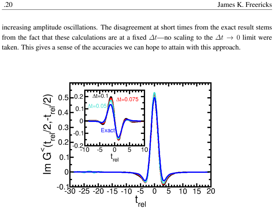
An introduction to many-body Green's functions in and out of equilibrium
Pith reviewed 2026-05-24 15:47 UTC · model grok-4.3
The pith
Dynamical mean-field theory extends to compute many-body Green's functions out of equilibrium.
A machine-rendered reading of the paper's core claim, the machinery that carries it, and where it could break.
Core claim
The paper establishes that dynamical mean-field theory, already successful for equilibrium properties, can be formulated on the Keldysh contour to calculate contour-ordered Green's functions for nonequilibrium situations, thereby providing graduate students with the concrete steps required to obtain spectral functions and other observables under time-dependent perturbations.
What carries the argument
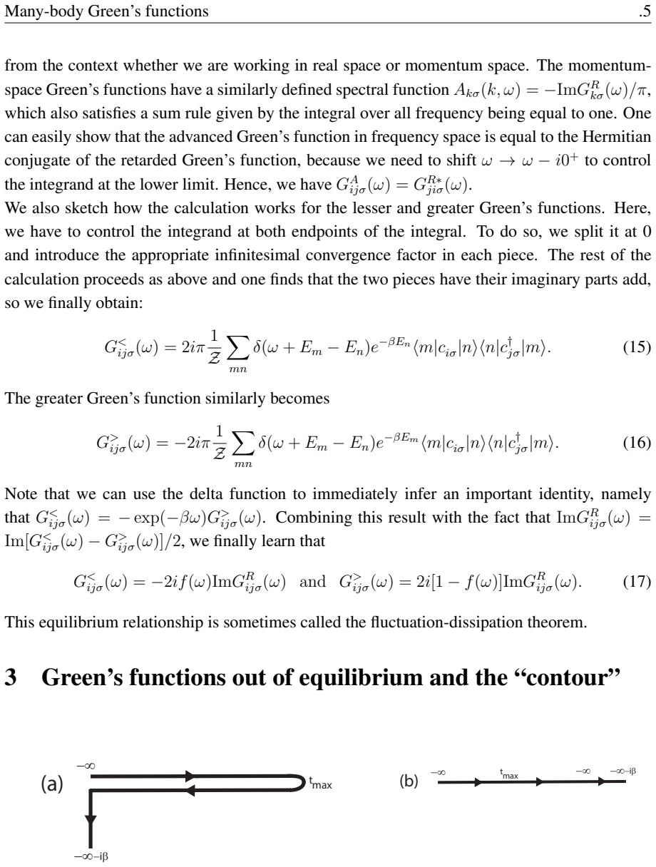
Contour-ordered Green's functions solved self-consistently within dynamical mean-field theory on the Keldysh contour.
If this is right
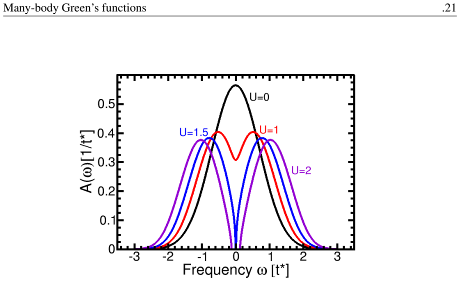
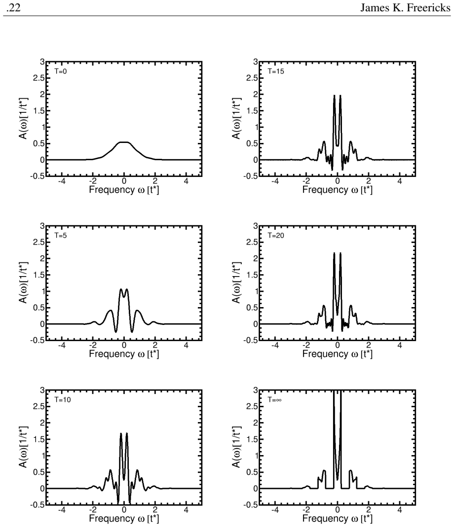
- Time-dependent spectral functions become computable for driven Hubbard-like models.
- Nonequilibrium DMFT supplies a consistent way to treat the impurity problem under time-dependent hybridization.
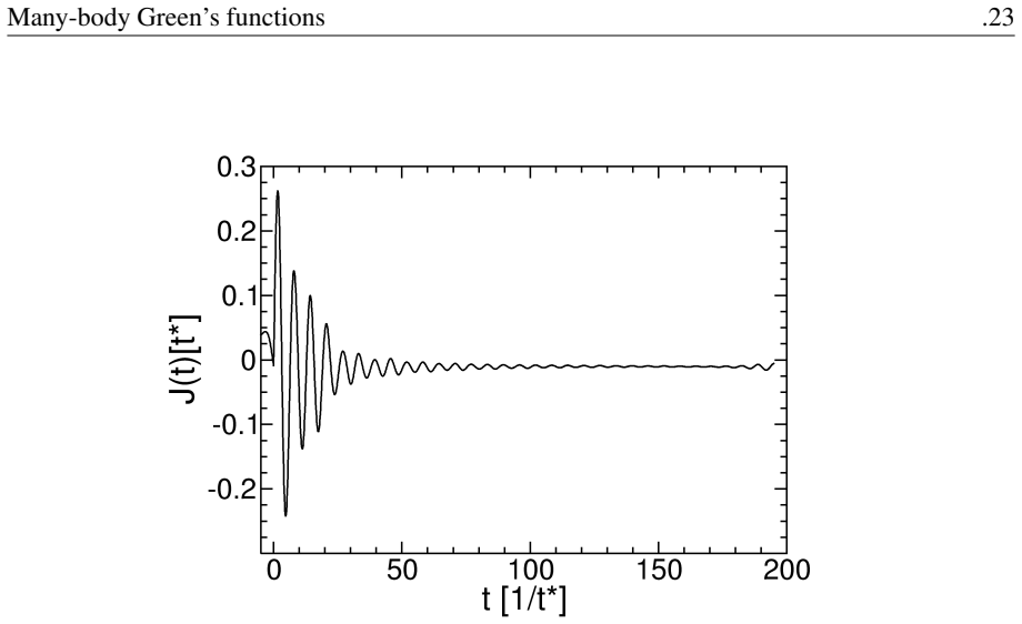
- Real-time response functions such as current or magnetization can be extracted directly from the Green's functions.
- The formalism recovers standard equilibrium DMFT as a special case.
Where Pith is reading between the lines
- The same contour technique might be combined with other impurity solvers beyond the ones presented here.
- Direct comparison with time-resolved photoemission data on specific materials would test practical accuracy.
- Extension to include nonlocal correlations could be examined by relaxing the DMFT locality assumption.
Load-bearing premise
Readers already possess a solid background in solid state physics and advanced quantum mechanics.
What would settle it
Explicit reduction of the nonequilibrium DMFT equations to the known equilibrium DMFT result when all external driving fields are switched off.
Figures
read the original abstract
This is an introductory chapter on how to calculate nonequilibrium Green's functions via dynamical mean-field theory for the Autumn School on Correlated Electrons: Many-Body Methods for Real Materials, 16-20 September 2019, Forschungszentrum Juelich. It is appropriate for graduate students with a solid state physics and advanced quantum mechanics background.
Editorial analysis
A structured set of objections, weighed in public.
Referee Report
Summary. This manuscript is an introductory chapter (Autumn School lecture notes) on calculating nonequilibrium Green's functions via dynamical mean-field theory. It targets graduate students with solid-state physics and advanced quantum mechanics backgrounds and presents standard DMFT techniques for equilibrium and nonequilibrium cases without introducing new derivations or results.
Significance. As pedagogical material, the work has value in accurately exposing established nonequilibrium DMFT methods to students. No novel claims, parameter-free derivations, or machine-checked results are present; significance rests on clarity and correctness of the exposition of standard techniques.
minor comments (1)
- The abstract states the target audience but the manuscript should explicitly list prerequisites (e.g., familiarity with Matsubara formalism or impurity solvers) at the start of the main text for clarity.
Simulated Author's Rebuttal
We thank the referee for the careful reading and the positive recommendation to accept the manuscript. We are pleased that the work is viewed as a useful pedagogical resource for the intended audience of graduate students.
Circularity Check
No significant circularity; purely pedagogical exposition
full rationale
The paper is explicitly an introductory lecture-note chapter presenting standard DMFT techniques for nonequilibrium Green's functions. It contains no novel derivations, quantitative predictions, or load-bearing claims that could reduce to self-definitions, fitted inputs, or self-citation chains. All content is expository of established material, with correctness depending on accurate presentation rather than any internal derivation chain. No steps meet the criteria for circularity.
Axiom & Free-Parameter Ledger
axioms (2)
- domain assumption Readers have solid state physics and advanced quantum mechanics background
- domain assumption Dynamical mean-field theory applies to nonequilibrium Green's functions in correlated systems
Lean theorems connected to this paper
-
IndisputableMonolith/Foundation/RealityFromDistinction.leanreality_from_one_distinction unclear?
unclearRelation between the paper passage and the cited Recognition theorem.
Nonequilibrium dynamical mean-field theory ... iterative algorithm
What do these tags mean?
- matches
- The paper's claim is directly supported by a theorem in the formal canon.
- supports
- The theorem supports part of the paper's argument, but the paper may add assumptions or extra steps.
- extends
- The paper goes beyond the formal theorem; the theorem is a base layer rather than the whole result.
- uses
- The paper appears to rely on the theorem as machinery.
- contradicts
- The paper's claim conflicts with a theorem or certificate in the canon.
- unclear
- Pith found a possible connection, but the passage is too broad, indirect, or ambiguous to say the theorem truly supports the claim.
Reference graph
Works this paper leans on
- [1]
-
[2]
A. A. Abrikosov, L. P. Gorkov, and I. E. Dzyaloshinski,Methods of Quantum Field Theory in Statistical Physics (Prentice Hall, New York, 1963)
work page 1963
-
[3]
J. M. Luttinger and J. C. Ward, Phys. Rev. 118, 1417 (1960)
work page 1960
- [4]
-
[5]
L. P. Kadanoff and G. Baym,Quantum statistical mechanics(Benjamin, New York, 1962)
work page 1962
-
[6]
L. .V . Keldysh, Zh. Eksp. Teor. Fiz. 47, 1515 (1964) in Russian; [Sov. Phys. JETP 20, 1018 (1965)]
work page 1964
-
[7]
A. Georges, G. Kotliar, W. Krauth, and M. J. Rozenberg, Rev. Mod. Phys. 68, 13 (1996)
work page 1996
-
[8]
J. K. Freericks, V . M. Turkowski, and V . Zlati´c, Phys. Rev. Lett. 97, 266408 (2006)
work page 2006
-
[9]
J. K. Freericks, Phys. Rev. B 77, 075109 (2008)
work page 2008
-
[10]
H. Aoki, N. Tsuji, M. Eckstein, M. Kollar, T. Oka, and P. Werner, Rev. Mod. Phys. 86, 779 (2014)
work page 2014
- [11]
- [12]
- [13]
- [14]
-
[15]
R. E. Peierls, Z. Phys. 80, 763 (1933)
work page 1933
-
[16]
A. Joura, Static and dynamic properties of strongly correlated lattice models under elec- tric fields (Dynamical mean field theory approach), Ph. D. thesis, Georgetown University (2014)
work page 2014
-
[17]
L. M. Falicov and J. C. Kimball, Phys. Rev. Lett. 22, 997 (1969)
work page 1969
- [18]
- [19]
- [20]
- [21]
-
[22]
Real-time formalism for studying the nonlinear response of ‘smart’ materials to an electric field,
J. K. Freericks, V . M. Turkowski, and V . Zlati ´c, “Real-time formalism for studying the nonlinear response of ‘smart’ materials to an electric field,” inProceedings of the HPCMP Users Group Conference 2005, Nashville, TN, June 28–30, 2005 edited by D. E. Post (IEEE Computer Society, Los Alamitos, CA, 2005), pp. 25–34
work page 2005
- [23]
-
[24]
G. Stefanucci and R. van Leeuwen, Nonequilibrium many-body physics of quantum sys- tems: A modern introduction (Cambridge University Press, Cambridge, 2013)
work page 2013
-
[25]
J. K. Freericks and V . Zlati´c, Rev. Mod. Phys. 75, 1333 (2003)
work page 2003
-
[26]
Nonequilibrium dynamical mean-field theory of strongly correlated electrons,
V . Turkowski and J. K. Freericks, “Nonequilibrium dynamical mean-field theory of strongly correlated electrons,” in Strongly Correlated Systems: Coherence and Entan- glement, edited by J. M. P. Carmelo, J. M. B. Lopes dos Santos, V . Rocha Vieira, and P. D. Sacramento (World Scientific, Singapore, 2007), pp. 187–210
work page 2007
-
[27]
A. V . Joura, J. K. Freericks, and T. Pruschke, Phys. Rev. Lett.101, 196401 (2008)
work page 2008
-
[28]
J. K. Freericks and A. V . Joura, “Nonequilibrium density of states and distribution func- tions for strongly correlated materials across the Mott transition,” in Electron transport in nanosystems, edited by J. Bonca and S. Kruchinin (Springer, Berlin, 2008) pp. 219–236
work page 2008
- [29]
-
[30]
Nonlinear response of strongly correlated materials to large electric fields,
J. K. Freericks, V . M. Turkowski, and V . Zlati´c, “Nonlinear response of strongly correlated materials to large electric fields,” inProceedings of the HPCMP Users Group Conference 2006, Denver, CO, June 26–29, 2006, edited by D. E. Post (IEEE Computer Society, Los Alamitos, CA, 2006), pp. 218–226
work page 2006
- [31]
-
[32]
J. K. Freericks, H. R. Krishnamurthy and T. Pruschke, Phys. Rev. Lett. 102, 136401 (2009)
work page 2009
-
[33]
O P. Matveev, A. M. Shvaika, T. P. Devereaux, and J K. Freericks, Phys. Rev. Lett. 122, 247402 (2019)
work page 2019
-
[34]
A. M. Shvaika and J. K. Freericks, Cond. Mat. Phys. 15, 43701 (2012); unpublished
work page 2012
-
[35]
Y . Chen, Y . Wang, C. Jia, B. Moritz, A. M. Shvaika, J. K. Freericks, and T. P. Devereaux, Phys. Rev. B 99, 104306 (2019)
work page 2019
discussion (0)
Sign in with ORCID, Apple, or X to comment. Anyone can read and Pith papers without signing in.