REVIEW 4 major objections 4 minor 1 cited by
Dueling Posterior Sampling for Preference-Based Reinforcement Learning
T0 review · 4 major / 4 minor · reviewed 2026-08-14 · deepseek-v4-flash
Pith's one-line read A reinforcement learning agent can converge to optimal behavior using only pairwise trajectory preferences, with no numerical rewards.
desk verdict First no-regret guarantee for preference-based RL, but the central proof has a load-bearing gap in Lemma 3; still worth serious refereeing. read the letter →
The pith
A machine-rendered reading of the paper's core claim, the machinery that carries it, and where it could break.
The reading
What carries the argument
The load-bearing object is the information ratio $\Gamma_i$, defined as the squared expected instantaneous one-sided regret divided by the mutual information that the observed preference outcome carries about the optimal policy: $\Gamma_i = \mathbb{E}_i[y^*_i - y_i]^2 \,/\, I_i(\pi^*; (\pi_{i2}, \tau_{i1}, \tau_{i2}, x_{i2} - x_{i1}, y_i))$. The argument bounds this ratio asymptotically by $SA/2$: regret incurred by the second sampled policy is at most the information it reveals about which policy is optimal, and since the feature difference $x_i = x_{i2} - x_{i1}$ lives in $d = SA$ dimensions, the rank of the associated matrix $B^{(i)}$ is at most $d$. The other main ingredient is the Bayesian linear regression posterior with ridge covariance $M_i = \lambda I + \sum x_i x_i^T$ and sampling covariance $\beta_i(\delta)^2 M_i^{-1}$, which must be shown to concentrate around the true reward vector; this is done by combining a high-probability ellipsoid for the MAP estimate with a contradiction argument that every state-action pair is visited infinitely often.
What would settle it
Run DPS on a finite MDP where preferences are generated by a logistic link function with reward differences exceeding $[-1/2, 1/2]$; if measured cumulative regret is not sublinear (e.g., grows linearly or the policy does not approach the optimum), the central theorem's assumptions fail. More directly, fit the linear credit assignment model and check whether the label residual $\mathbb{E}[y_i - r^T(x_{i2}-x_{i1})]$ is zero-mean under the true preference generator.
Extended reading notes
Core claim
Under a linear link function, preferences are modeled as noisy measurements of the reward difference: $\mathbb{E}[y_i] = r^T(x_{i2} - x_{i1})$, with $y_i \in \{-1/2, 1/2\}$. DPS treats each episode as a duel between two policies sampled from the posterior; because both trajectories are rolled out, observing which wins gives one bit about the difference of their feature vectors. The paper proves three things: sampled dynamics and rewards converge in distribution to their true values; the information ratio for the one-sided regret is asymptotically bounded by $SA/2$; and combining these gives the regret rate $S\sqrt{2AT\log A}$ with probability $1-\delta$. The proof works through a Bayesian linear regression credit assignment model and an information-theoretic analysis of Thompson sampling adapted to preference feedback.
Load-bearing premise
The theorem assumes users' preferences are generated by a linear link function: the probability of preferring one trajectory over the other is exactly proportional to the difference in their total rewards, plus zero-mean noise; if real preferences follow a logistic or other nonlinear model, the Bayesian linear regression posterior is misspecified and the proof no longer applies.
Editorial extensions
If this is right
- DPS is the first preference-based RL algorithm with a regret guarantee: if the theorem holds, expected regret grows as $S\sqrt{2AT\log A}$, which is sublinear in $T$, so the algorithm converges to the optimal policy.
- DPS is asymptotically consistent: the sampled policies converge in distribution to the optimal policy as iterations increase, meaning exploration eventually concentrates on optimal behavior.
- If the transition dynamics are known a priori, the same proof gives a finite-time regret bound, since the asymptotic step in the argument only comes from learning the dynamics.
- The authors conjecture that the proof method extends to other asymptotically consistent credit assignment models, which would make DPS a general template for preference-based RL.
Reading between the lines
- A direct consequence the authors do not spell out: the per-state-action factor $S$ and per-action factor $\sqrt{A}$ in the regret rate suggest that the algorithm's exploration cost is essentially the cost of identifying rewards in all $SA$ state-action pairs, so the bound is tight in $S$ and $A$ up to log factors.
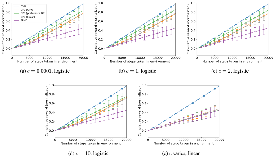
- The linear-link assumption is stronger than the experiments suggest; because the simulations generate preferences with a logistic model and DPS still works, it is plausible the regret bound survives for noisy logistic preferences if reward differences are small enough to approximate the linear link.
- One testable extension would be to replace the binary preference bit with a $k$-ary or continuous preference strength; the information-ratio argument should carry over since mutual information only increases with richer feedback, likely lowering regret.
Signed reviews
Editorial analysis
A structured set of objections, weighed in public.
Referee Report
Summary. The paper proposes Dueling Posterior Sampling (DPS), a preference-based reinforcement learning algorithm that maintains Bayesian posteriors over both transition dynamics and a state-action reward model, and at each episode draws two posterior samples, computes the corresponding optimal policies via value iteration, and rolls them out to obtain a pairwise trajectory preference. The authors prove an asymptotic Bayesian no-regret guarantee of S√(2AT log A) for DPS under a Bayesian linear regression credit assignment model, and support the theory with experiments in RiverSwim, random MDPs, and Mountain Car. The proof adapts the information-ratio framework of Russo and Van Roy (2016) and the dueling-bandit Self-Sparring idea of Sui et al. (2017).
Significance. If the main theorem were fully established, this would be the first regret guarantee for preference-based reinforcement learning, a contribution of clear value to a growing field. The paper is well structured, the empirical study is reasonably thorough, and the code is publicly available. The information-theoretic treatment of credit assignment for trajectory-level preferences is an interesting technique that could inform later work. However, the proof as written contains a load-bearing gap in the asymptotic consistency argument, so the central claim is not yet rigorously supported.
major comments (4)
- [Appendix A.1, Lemma 3] The uniform exploration lower bound is not justified. The proof defines v := h/ρ_1, where ρ_1 = max_π V(p̃, r_1, π) is the expected number of visits to the target state-action pair under the optimal policy for reward vector r_1. It then argues that ρ_1 is continuous on the compact transition simplex, so v lies in [v_min, v_max] with v_min > 0. This is incorrect: ρ_1 can be arbitrarily small, and is exactly zero for sampled dynamics under which the target pair is unreachable. For such p̃, v is undefined or infinite rather than an element of a compact interval with a positive lower bound. Consequently the probability of the event {r̃_1 ≥ v max_j r̃_j} can decay without limit as v grows, and the claimed existence of a uniform ρ > 0 over all p̃ does not follow. Since Proposition 1, Theorem 1, and Theorem 3 all depend on Lemma 3, the central no-regret claim is not established by the proof as written.
- [Appendix A.1, Lemma 3] The statement 'Such a policy always takes action a in state s' is not implied by π_vi(p̃, r_1) maximizing the expected number of visits to (s,a). In a finite-horizon MDP, a policy that occasionally selects a different action in s can return to s and thereby accumulate more expected visits to (s,a) than a policy that always takes action a in s. Thus the mechanism by which DPS is claimed to reach an unvisited state-action pair infinitely often is not rigorously established even if the uniform lower bound on sampling π_vi(p̃, r_1) were valid.
- [Section 3, Assumption 2 and Section 4.1] The linear link function model has a domain inconsistency. The paper defines g_lin(x) = c x for x ∈ [-1/(2c), 1/(2c)] and then says 'Without loss of generality, we set c = 1 by subsuming c into r.' This is not without loss of generality: the domain constraint depends on c, and after absorbing c into r the range constraint becomes r^T(x_{i2} - x_{i1}) ∈ [-1/2, 1/2]. Assumption 4 only bounds ||r||_2 ≤ S_r, which does not imply this range for all trajectory pairs (e.g., ||x_{i2} - x_{i1}||_1 can be as large as 2h). The stated assumptions therefore allow preference probabilities outside [0,1], so the theoretical model is not always well defined. The authors should either add an explicit assumption that realized reward differences lie in the valid range or discuss how the analysis extends when the linear link is only an approximation.
- [Appendix A.1, Lemma 11] The proof that β_i(δ)^2 / λ_d^(i) converges to zero in distribution is not rigorous. The argument shows that, under a contradiction hypothesis, λ_d^(i) grows at least linearly in expectation over a subsequence of indices, but expectation bounds do not imply high-probability or almost-sure growth. The final case analysis, which rules out non-convergence in probability by applying the same argument 'over time indices where β_i^2/λ_d ≥ ε', is asserted rather than proved; non-convergence in probability does not by itself guarantee that those indices form a non-decaying subset along which the same expected-growth argument can be applied. Since Proposition 2 and Theorem 1 rely on Lemma 11, this is another load-bearing gap in the proof.
minor comments (4)
- [Appendix A.1, Lemma 3] The symbol v is used both for the threshold h/ρ_1 and for eigenvectors v_j^(i) of M_i, which makes the proof harder to follow. Please rename one of them.
- [Appendix A.1, Lemma 5] The lemma states the hypothesis as β_i(δ)^2 / λ_d^(i) → 0, but the proof says 'By assumption, λ_d^(i)/β_i(δ)^2 → ∞'; these are equivalent, but the direction of the convergence in distribution should be stated consistently throughout.
- [Appendix A.1, Proposition 2] The statement 'the sampled rewards ˜ri1, ˜ri2 converge in distribution to the true reward parameters, ˜ri1, ˜ri2 D −→ r' contains a typo: the variables are repeated after the comma. It should read '˜ri1, ˜ri2 D −→ r'.
- [Section 5, Lemma 17] The proof of Lemma 17 says the numerator 'does not depend upon the action xi1' and is thus unaffected by the drifting distribution of π_i1; this is true for the expectation, but the conditioning history H_i^(2) includes π_i2 and the comparison trajectory τ_i1, so please clarify that the conditioning is on the full history and that the cancellation in (40) holds under the martingale structure used in Lemma 12.
Circularity Check
Lemma 3's proof invokes Lemma 1, whose premise is the very infinite-visitation conclusion Lemma 3 must prove; Proposition 1 and Theorem 3 inherit this circular step.
-
other
[Appendix A.1, Lemma 3 (proof of infinite visitation), final paragraph; cross-ref Lemma 1]
"Lemma 1. If every state-action pair is visited infinitely-often, then the sampled transition dynamics parameters converge in distribution to their true values... In case b), due to Lemma 1, the transition dynamics parameters for state-actions along the path to s converge to their true values (intuitively, the algorithm knows how to reach s)."
Lemma 3's goal is exactly to prove that every state-action pair is visited infinitely-often. Lemma 1 is the conditional statement that this same global visitation property implies convergence of the sampled dynamics. The proof of Lemma 3 invokes Lemma 1 to assert that dynamics along a path to s converge, thereby using the conclusion of Lemma 3 as an input to Lemma 1. As written, this is a circular argument: the premise of Lemma 1 is the proposition that Lemma 3 is supposed to establish. Since Proposition 1, Theorem 1, and Theorem 3 all depend on Lemma 3, the central no-regret guarantee inherits this circular dependency. A local version of the concentration argument could repair the step, but the manuscript does not state or prove such a version.
full rationale
The main regret derivation is not circular in the usual 'fitted input as prediction' sense: Assumptions 2-4 are stated modeling assumptions, the Bayesian linear regression posterior is not fit to the target regret, and the concentration and ellipsoid arguments are imported from Abbasi-Yadkori et al. (2011) and Russo and Van Roy (2016), which are independent external results. The self-citations to Sui et al. (2017) are for algorithmic inspiration only and are not used as a load-bearing theorem. However, there is one load-bearing circular step in the consistency proof. Lemma 3 is supposed to establish that every state-action pair is visited infinitely often; to handle the case where an infinitely visited set contains a path to s, the proof invokes Lemma 1, which is explicitly conditioned on the global statement 'every state-action pair is visited infinitely-often', the very conclusion being proved. As written, this assumes the target result. Proposition 1, Theorem 1, and Theorem 3 each depend on this chain, so the paper's headline regret rate is partially circular in its proof, even though it is not equivalent by construction to the assumptions. Separately, the uniform lower bound v = h/rho1 >= v_min > 0 asserted in Lemma 3 is not justified when rho1 can tend to zero on the boundary of the transition simplex; that is a non-circular correctness gap, and it further undermines the proof as written. Score 5 reflects one central circular dependency while acknowledging that most of the analysis has independent content.
Assumptions & free parameters
free parameters (5)
- Regularization parameter λ =
λ ≥ 1 (theoretically); tuned in experiments (e.g., 0.1, 1, 10)
- Sub-Gaussian constant R =
R ≤ 1
- Reward norm bound S_r =
assumed known
- Failure probability δ =
chosen in (0,1)
- Dirichlet prior hyperparameters α_{jk,0} =
user-defined, set to 1 in RiverSwim/random MDP experiments; 0.0005 in Mountain Car
assumptions (9)
- domain assumption Trajectory utility decomposes additively over state-action rewards: r(τ) = Σ r(s_t,a_t).
- domain assumption Preference probabilities are generated by an odd, non-decreasing link function of reward differences; theory uses linear link g_lin(x)=c x, with c subsumed into r (c=1).
- domain assumption Label noise η_i is conditionally R-sub-Gaussian with zero mean.
- domain assumption The reward vector is bounded: ||r||_2 ≤ S_r for known S_r.
- domain assumption State transitions are fully observed and modeled with Dirichlet-multinomial priors.
- standard math Abbasi-Yadkori et al. Theorem 2 (self-normalized martingale concentration) holds.
- standard math Russo and Van Roy information ratio facts (Fact 9 and Fact 10) and entropy/mutual information chain rules hold.
- standard math Value iteration over the finite set of deterministic policies returns an optimal policy for the sampled MDP.
- ad hoc to paper Unidentifiable reward directions can be ignored without loss of generality.
Cite this review
Pith. "Pith review of Dueling Posterior Sampling for Preference-Based Reinforcement Learning." pith.science (2026). https://pith.science/paper/ETMNHDK7
@misc{pith2026190801289,
  author       = {Pith},
  title        = {Pith review of: Dueling Posterior Sampling for Preference-Based Reinforcement Learning},
  year         = {2026},
  howpublished = {\url{https://pith.science/paper/ETMNHDK7}},
  note         = {Machine review of arXiv:1908.01289}
}
read the original abstract
In preference-based reinforcement learning (RL), an agent interacts with the environment while receiving preferences instead of absolute feedback. While there is increasing research activity in preference-based RL, the design of formal frameworks that admit tractable theoretical analysis remains an open challenge. Building upon ideas from preference-based bandit learning and posterior sampling in RL, we present DUELING POSTERIOR SAMPLING (DPS), which employs preference-based posterior sampling to learn both the system dynamics and the underlying utility function that governs the preference feedback. As preference feedback is provided on trajectories rather than individual state-action pairs, we develop a Bayesian approach for the credit assignment problem, translating preferences to a posterior distribution over state-action reward models. We prove an asymptotic Bayesian no-regret rate for DPS with a Bayesian linear regression credit assignment model. This is the first regret guarantee for preference-based RL to our knowledge. We also discuss possible avenues for extending the proof methodology to other credit assignment models. Finally, we evaluate the approach empirically, showing competitive performance against existing baselines.
Figures


Figures from the paper (4 more)


Forward citations
Cited by 1 Pith paper
-
Thompson Sampling in Online RLHF with General Function Approximation
A model-free posterior sampling algorithm for online RLHF is shown to achieve O(sqrt(T)) regret when the completed function class has low Bellman eluder dimension.
Reference graph
Works this paper leans on
-
[2]
Then, asymptotically bound the one-sided regret rate forπi2 (Appendix A.2)
Assume that in each iteration i, policyπi1 is drawn from a fixed distribution while policyπi2 is selected by DPS. Then, asymptotically bound the one-sided regret rate forπi2 (Appendix A.2)
-
[3]
Then, asymptotically bound the one-sided regret rate forπi2 (Appendix A.3)
Assume that policy πi1 is drawn from a drifting but converging distribution while policyπi2 is selected by DPS. Then, asymptotically bound the one-sided regret rate forπi2 (Appendix A.3). Finally, Appendix A.4 combines these results to asymptotically bound the expected regret rate. A.1 ASYMPTOTIC CONSISTENCY OF DPS We show asymptotic consistency ofDPS in ...
work page 2010
-
[4]
We prove the desired statement by contradiction: assume that there is nob< ∞ such that||ˆrn||2≤b for alln. Then, the sequence ˆr1, ˆr2,... must have a subsequence indexed by(ni) such that limi−→∞||ˆrni||2 =∞. Consider the sequence of unit vectors ˆrni ||ˆrni||2 . This sequence lies within the compact set of unit vectors in Rd, and so it must have a conver...
work page 2011
-
[6]
For v∈ Rd such that||v||2 = 1,v∈Sk for somek∈{ 1,...,K }, and
-
[7]
If v1,v2∈Sk, then||v1−v2||<ε . We will show that there exists a sequence (ni)∈ N such thatv(ni) d ∈ Sk for fixed k∈{ 1,...,K }, with the events v(ni) d ∈ Sk corresponding to the indices (ni) occurring at some non-decaying frequency. Then, by appropriately choosingε, we will use (36) and the mutual proximity of the vectorsv(ni) d to show thatλ(n) d increase...
work page 2016
-
[8]
To inferr, we approximate eachr(τi) with its preference labelyi
As before, we use r(˜s) to denote the true utility of state-action ˜s, withr(τ) being trajectoryτ’s total utility along the state-action pairs it encounters. To inferr, we approximate eachr(τi) with its preference labelyi. We place a Gaussian process prior upon the rewards r: r∼GP (µr,Kr), where µr ∈ Rd is the prior mean and Kr∈ Rd×d is the prior covarian...
work page 2005
-
[9]
Prove that DPS is asymptotically-consistent, that is, over time, the probability that DPS selects the optimal policy approaches 1 (Appendix A.1)
-
[10]
Then, asymptotically bound the one-sided regret forπi2 (Appendix A.2)
Assume that in each iteration i, policyπi1 is drawn from a fixed distribution while policyπi2 is selected by DPS. Then, asymptotically bound the one-sided regret forπi2 (Appendix A.2)
Show all 12 references
-
[11]
Then, asymptotically bound the one-sided regret forπi2 (Appendix A.3)
Assume that policy πi1 is drawn from a drifting but converging distribution while policyπi2 is selected by DPS. Then, asymptotically bound the one-sided regret forπi2 (Appendix A.3). Notably, this proof outline does not depend upon any specific credit assignment model definition...
-
[12]
The information-theoretic perspective used to prove 2) and 3) likely applies to a wide class of credit assignment models
depends mainly upon continuity arguments. The information-theoretic perspective used to prove 2) and 3) likely applies to a wide class of credit assignment models. For instance, recent work has applied the bandit analysis framework in Russo and Van Roy (2016) to bandits with r...
2016
-
[13]
Under this assumption, one can show that applying the martingale techniques yields the following variant of (65): n∑ i=1 2∑ j=1 xT ij ( λI + i−1∑ s=1 xsxT s )−1 xij
Thus, only differences between compared trajectory feature vectors yield information about the rewards. Under this assumption, one can show that applying the martingale techniques yields the following variant of (65): n∑ i=1 2∑ j=1 xT ij ( λI + i−1∑ s=1 xsxT s )−1 xij. (66) Th...
2016
-
[248]
ACM, 2005. S. Y . Ramamohan, A. Rajkumar, and S. Agarwal. Dueling ban- dits: Beyond Condorcet winners to general tournament so- lutions. In Advances in Neural Information Processing Sys- tems, pages 1253–1261, 2016. K. Raman, T. Joachims, P. Shivaswamy, and T. Schnabel. Sta- b...
2005
Reviewed August 14, 2026 · model on record in the stance chip above.
Discussion (0). Continue with ORCID to comment.