REVIEW 3 major objections 4 minor 1 cited by
Latent Space Modelling of Hypergraph Data
T0 review · 3 major / 4 minor · reviewed 2026-08-14 · deepseek-v4-flash
Pith's one-line read The paper proposes a latent space model for non-simplicial hypergraphs, built from per-order Cech skeletons with Bernoulli noise, whose likelihood is cheap to evaluate and whose posterior can be sampled with MCMC under Bookstein…
desk verdict A genuine new latent-space model for non-simplicial hypergraphs with a cheap likelihood, but the MCMC ignores the model's ordering constraint and the abstract oversells; still worth refereeing after fixes. read the letter →
The pith
A machine-rendered reading of the paper's core claim, the machinery that carries it, and where it could break.
The reading
What carries the argument
The key object is the non-simplicial random geometric hypergraph (nsRGH): the union over k of the order-k skeletons of Cech complexes with per-order radii r_2 < r_3 < ... < r_K, where each Cech complex records all subsets of nodes whose radius-r_k balls have a common intersection. The argument rides on the equivalence that a k-set of latent points becomes a hyperedge exactly when its smallest enclosing ball has radius at most r_k, which turns hyperedge checking into miniball computations and makes the likelihood evaluable by counting hyperedge matches and mismatches rather than enumerating all possible hyperedges.
What would settle it
Fit the model to a hypergraph containing a high-degree 3-star—one central node in many order-3 hyperedges whose other two nodes share no pairwise hyperedge—and compare the observed star count with the posterior predictive count under the fitted geometry; if the observed count lies far outside the predictive range, the thresholded-ball premise is not generating the data.
Extended reading notes
Core claim
The central claim is that non-simplicial hypergraph data can be modelled by a non-simplicial random geometric hypergraph built from Cech complexes: for each order k, a separate radius r_k is used, and only hyperedges of exactly order k are selected from the k-skeleton. Taking the union over k removes the simplicial constraint, and independent Bernoulli modifications give the model support on all hypergraphs and a Hamming-distance likelihood that is a product of Bernoulli factors. Conditional on latent coordinates, the geometry is deterministic, so the latent positions carry the structure and the modification probabilities absorb discrepancies. With normal priors on coordinates, the model implies exchangeability of nodes and a higher-order transitivity in which subsets of a latent geometric hyperedge are likely to be present even when they are not logically required.
Load-bearing premise
The load-bearing premise is that a hyperedge of order k forms exactly when the k latent points all lie inside some ball of radius r_k, so that real-world higher-order interactions are well approximated by a purely geometric overlap threshold; if the true process is non-geometric or non-exchangeable, the latent representation is a misspecified projection.
Editorial extensions
If this is right
- Hypergraphs gain the same visualisation as latent space graphs: posterior mean coordinates place centrally connected actors at the centre and peripheral nodes at the edge, as demonstrated on the Star Wars and coauthorship datasets.
- Predictive inference for new nodes follows naturally: simulate coordinates from the fitted normal, read off the induced hyperedges, and estimate degree or motif distributions for a next wave of nodes.
- The degree distribution of order-2 hyperedges is exactly Binomial and order-3 hyperedges are approximately Poisson (Lemma 4.1 and Theorem 4.1), connecting model parameters directly to observable degree summaries.
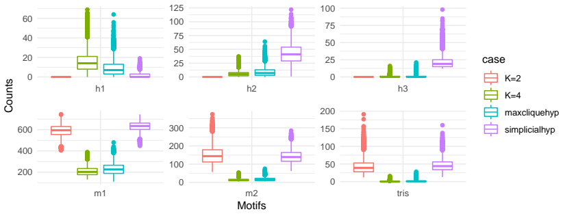
- Per-order radii plus directed modification probabilities let the same framework express very different regimes, such as dense pairwise edges with sparse triangles, and broad comparison shows the model covers a wider range of motif counts than two existing hypergraph baselines.
Reading between the lines
- A direct extension, not pursued in the paper, would replace the Cech skeleton with a Vietoris-Rips construction so that an order-k hyperedge is present when all pairwise balls intersect; the authors note this would scale better in K, and a natural test is whether posterior predictive motif counts change materially across the two complexes.
- Because the likelihood treats the geometry as a deterministic incidence pattern with independent flips, the same framework could accommodate weighted or repeated hyperedges by letting the modification probabilities depend on multiplicity, which the paper leaves open.
- The geometric core can only express star-like structures up to a limit set by the latent dimension, so for datasets with very high-degree centres the fitted noise parameters, not the latent positions, will carry the explanatory burden; checking the posterior of the modification probabilities would reveal when the geometric interpretation is strained.
Editorial analysis
A structured set of objections, weighed in public.
Referee Report
Summary. The paper proposes a Bayesian latent space model for non-simplicial hypergraph data. Hyperedges are generated as the union of order-k skeletons of Čech complexes with per-order radii r_k, subject to r_k > r_{k-1}, and then each hyperedge indicator is independently flipped with a small probability. This construction yields likelihoods (10) and (13) that are inexpensive to evaluate, and the authors use Bookstein coordinates to remove rotation, translation, and scaling non-identifiability. Posterior sampling is carried out by a Metropolis-within-Gibbs scheme, Section 4 derives degree-distribution results, and simulation and real-data analyses (Star Wars co-occurrence and a statistician coauthorship subset) illustrate the framework. The central claim is that this is the first computationally tractable latent-position model for non-simplicial hypergraphs.
Significance. The modeling idea is natural and original, and it is developed in a mostly coherent way. The likelihood is derived from the generative mechanism rather than fitted to an external benchmark, which is appropriate for model-based inference; the connection to Čech-complex skeletons is a useful bridge from computational topology to statistical network analysis. The paper also includes predictive degree-distribution studies and two real-data applications, and it gives detailed appendices on initialization, implementation, and misspecification. If the technical problems below are fixed, the framework would be a valuable contribution to the hypergraph and latent-space network literature. The current version, however, contains errors in the theoretical degree-distribution results and a mismatch between the model's support and the MCMC implementation.
major comments (3)
- [Section 5.1, Algorithm 3, Eq. (22)] The MCMC scheme does not enforce the ordering constraint r_k > r_{k-1} required by Definition 3.1. In Algorithm 3 each r_k is proposed independently as r_k + epsilon_r, and the acceptance probability in Eq. (22) uses only the independent exponential prior p(r|lambda). The chain can therefore visit parameter values for which the induced hypergraph is simplicial, meaning it samples from a larger model than the one defined in Section 3.2. This is not purely cosmetic: the non-simplicial claims in Sections 7.1 and 7.2 are made for the ordered-radius model. A reparameterization to increments delta_k = r_k - r_{k-1} > 0, or an indicator restricting the prior/support to the ordered set, would fix the problem.
- [Theorem 4.1(2), Eq. (20)] The displayed Poisson rate in Eq. (20) is wrong. There are C(N-1,2) hyperedges e3 incident to node i, and Eq. (20) multiplies each of those summands by C(N-1,2). The resulting rate is C(N-1,2)^2 times the per-hyperedge probability rather than C(N-1,2) times it. This algebraic error directly affects the theoretical claim and the comparison made in Figure 11. The binomial coefficient should be removed from the summand, or the entire sum should be replaced by C(N-1,2) times the common per-hyperedge success probability.
- [Theorem 4.1(1)-(2), Appendix F.3] The theorem states a marginal degree distribution after integrating over the latent positions, but the indicators of hyperedges incident to node i are not independent conditional only on (phi, Sigma, r). Conditional on the latent position u_i, the indicators are independent, but u_i is itself random; the marginal degree of node i is therefore a mixture of Binomials (and, for k=3, a mixture of Poisson-binomials), not a single Binomial or Poisson law. The proof's phrase 'given conditioning on i' does not remove this dependence; conditioning on the full latent configuration U would, but then the statement should be explicitly conditional on U. This is a load-bearing issue because Section 4 presents these distributions as exact results and Section 7.2 relies on them for the real-data comparison.
minor comments (4)
- [Abstract and Section 5] The abstract promises a 'delayed-acceptance MCMC scheme,' but Section 5 describes only a Metropolis-Hastings-within-Gibbs sampler with no delayed-acceptance step; please align the abstract with the actual algorithm.
- [Section 3.4] The title 'Can we improved model flexibility?' is a typo, and the phrase 'for k = 2, 4,..., K - 1' should presumably be 'for k = 2, 3, ..., K - 1'.
- [Equation (11)] Equation (11) appears to contain a typesetting error: 'Sigma mu ~ W^-1(Phi, nu)' should presumably be 'Sigma ~ W^-1(Phi, nu)'.
- [Section 6.2] The text 'we being by simulating a hypergraph' should read 'we begin by simulating a hypergraph'.
Circularity Check
No significant circularity: the nsRGH likelihood is derived from the stated generative mechanism, self-citations are not load-bearing, and held-out predictive checks are genuine.
full rationale
The paper's central derivation chain is self-contained. Definition 3.1 defines the non-simplicial random geometric hypergraph as the union of k-skeletons of Cech complexes with ordered radii; Algorithm 1/2 and equations (10)/(13) construct the likelihood directly as a product of Bernoulli modification probabilities, so there is no fitted input renamed as a prediction. The only self-citations are contextual: Lunagómez et al. (2017) is cited as related work, and the remark about likelihood monotonicity cites Lunagómez et al. (2019, proof of Proposition 3.1), but the monotonicity claim is evident from (10) itself when 0 < phi_k < 1/2, so the citation is not load-bearing. Bookstein coordinates are an identifiability convention, not an imported uniqueness theorem. The Section 7.2 comparison of theoretical and observed degree distributions uses fitted parameters and is an in-sample diagnostic, not a claimed prediction; the actual predictive check targets the next sampling wave, which is not used in fitting. The MCMC issue raised by the skeptic (unconstrained r proposals) is a potential implementation/correctness gap relative to Definition 3.1, but it is not circularity: the model and sampler are not defined in terms of the paper's conclusions. No step in the derivation reduces to its own inputs by construction.
Assumptions & free parameters
free parameters (5)
- Per-order radii r_k (k=2,...,K) =
e.g., rhat=(0.13,0.16) in Section 6.2; estimated per dataset
- Flip probabilities phi_k or psi_k^(0), psi_k^(1) =
e.g., psihat=(0.0058,0.0014),(0.0057,0.0035) in Section 6.2
- Latent mean mu =
e.g., muhat=(-0.13,0.44) in Section 6.2
- Latent covariance Sigma =
e.g., Sigmahat=[[0.14,-0.0039],[-0.0039,0.078]] in Section 6.2
- Latent dimension d =
2 in most examples; 3 in one simulation case
assumptions (5)
- domain assumption Latent coordinates u_i are iid N(mu, Sigma).
- domain assumption Hyperedges of each order occur independently conditional on U and r.
- standard math An order-k hyperedge is present iff the k latent points lie in a ball of radius r_k.
- standard math Poisson approximation for sums of dependent Bernoulli trials is valid when p3 is small.
- standard math Bookstein coordinates remove translation, rotation, and scaling non-identifiability.
invented entities (2)
-
Non-simplicial random geometric hypergraph (nsRGH), union of k-skeletons D^(k)_{r_k}
-
Hyperedge flip noise (phi_k or psi_k^(0), psi_k^(1))
Cite this review
Pith. "Pith review of Latent Space Modelling of Hypergraph Data." pith.science (2026). https://pith.science/paper/7Q2B6YBH
@misc{pith2026190900472,
  author       = {Pith},
  title        = {Pith review of: Latent Space Modelling of Hypergraph Data},
  year         = {2026},
  howpublished = {\url{https://pith.science/paper/7Q2B6YBH}},
  note         = {Machine review of arXiv:1909.00472}
}
read the original abstract
The increasing prevalence of relational data describing interactions among a target population has motivated a wide literature on statistical network analysis. In many applications, interactions may involve more than two members of the population and this data is more appropriately represented by a hypergraph. In this paper, we present a model for hypergraph data which extends the well established latent space approach for graphs and, by drawing a connection to constructs from computational topology, we develop a model whose likelihood is inexpensive to compute. A delayed-acceptance MCMC scheme is proposed to obtain posterior samples and we rely on Bookstein coordinates to remove the identifiability issues associated with the latent representation. We theoretically examine the degree distribution of hypergraphs generated under our framework and, through simulation, we investigate the flexibility of our model and consider estimation of predictive distributions. Finally, we explore the application of our model to two real-world datasets.
Figures


Figures from the paper (16 more)


Forward citations
Cited by 1 Pith paper
-
Modeling Hypergraphs with Diversity and Heterogeneous Popularity
New generative hypergraph model based on determinantal point processes, with consistency and asymptotic normality guarantees for maximum likelihood estimates.
Reference graph
Works this paper leans on
-
[1]
Sample i1 with probability p(i1) = N−i1 ∑N−1 i=1 (N−i) , for i1 = 1,..., (N− 1)
-
[2]
A similar procedure can be used for arbitrary k
Sample i2|i1 with probability p(i2|i1) = 1 N−i1 , for i2 = (i1 + 1),...,N . A similar procedure can be used for arbitrary k. Note that this procedure ignores the dependence between samples since, once a hyperedge is sampled, the remaining hyperedges are sampled from a subset of hyperedges of size (N k ) − 1. However, we expect this effect to be negligible ...
work page 2012
-
[3]
Apply MDS to D to obtain coordinates U0∈ RN×d
-
[4]
The radii r depend on the scale of U, and so they are initialised in terms of U0
Specify the index of the anchor points, and transform U0 onto Bookstein coordinates (see Appendix A). The radii r depend on the scale of U, and so they are initialised in terms of U0. Given the initial latent coordinates, r0 is chosen to be the minimum radius which induces all edges that are present in hN,K. The noise parameters ψ(0) andψ(1) are initialis...
-
[5]
Let A∈ RN×N denote a weighted adjacency matrix. Fori,j ∈{ 1, 2,...,N }, if{i,j} are connected by a hyperedge - let A(i,j) = 1 if{i,j} are only connected by a hyperedge of order k = 2, - let A(i,j) =λ if{i,j} are connected by a hyperedge of order k> 2
-
[6]
Find the distance matrix D∈ RN×N, where D(i,j) is the shortest path between nodes{i,j} in the weighted graph determined by A. For i =j, let D(i,j) = 0
- [9]
-
[10]
-Sample u∗ i∼N (µ∗, Σ∗) for i = 1, 2,...,N
While n<N smp -Sample µ∗∼N (mµ, Σµ) and Σ∗∼W−1(Φ,ν ). -Sample u∗ i∼N (µ∗, Σ∗) for i = 1, 2,...,N . LetU∗ be the N×d matrix whose ith row is u∗ i . -Given initialr0, determine the hypergraph gN,K(U∗,r0). -Let g∗ N,K by the hypergraph obtained by modifying gN,K(U∗,r0) with noise ψ(0) 0 andψ(1) 0 -Calculate T ( g∗ N,K ) . -If|T (hN,K)−T (g∗ N,K)|<ϵ Accept sa...
Show all 30 references
-
[11]
To initialise the parameters µ and Σ we use an ABC scheme (see Marin et al
Let µ0 and Σ0 be the average of Nsmp samples. To initialise the parameters µ and Σ we use an ABC scheme (see Marin et al. (2012) for an overview). In this scheme we first sampleµ and Σ from their priors. Conditional on these samples, we then sample a hypergraph. By comparing su...
2012
-
[12]
and uB 2 = (uB 21,uB
-
[13]
Determine U0 by applying Algorithm 4
-
[14]
Let initial radii r0 be the smallest radii which induce all hyperedges observed in hN,K, conditional on U0
-
[15]
Sample ψ(0) 0 andψ(1) 0 from their prior distributions
-
[16]
E Practicalities To implement the MCMC scheme given in Algorithm 3 there are a number of practical con- siderations we must address
Sample µ0 and Σ0 by applying Algorithm 5. E Practicalities To implement the MCMC scheme given in Algorithm 3 there are a number of practical con- siderations we must address. In this section we comment on these where, in E.1 we discuss an approach for determining the presence ...
2010
-
[17]
Determine the smallest enclosing ball B for the coordinates{ui1,ui2,...,u ik}
-
[18]
If the radius of B is less than rk, the hyperedge ek ={i1,i 2,...,i k} is present in the hypergraph. To compute the smallest enclosing ball we can rely on the the miniball algorithm (see Section 3.2 of Edelsbrunner and Harer (2010)), which may be also be referred to as the min...
2010
-
[19]
Set σ1 =ek and σ2 =∅
-
[20]
(2008), and for efficient implementation of the ˇCech complex we rely on the GUDHI C++ library (The GUDHI Project (2015))
if σ1 =∅, compute the miniball B of σ2 else choose u∈σ1 -Calculate the miniball B which contains the points σ1\u in its interior and the points σ2 on its boundary -if u /∈B, then set B to be the miniball B which contains the points σ1\u in its interior and the points σ2∪u on i...
2008
-
[21]
All nodes equally likely to form connections βi =−1.4 for i = 1, 2,...,N
-
[22]
LetUB denote the Bookstein coordinates andU denote the untransformed coordinates
to be ( −1/2, 0) and (1/2, 0), respectively. LetUB denote the Bookstein coordinates andU denote the untransformed coordinates. Then UB is given by UB =cR(U−b) = 1√ (uB 21−uB 11)2 + (uB 22−uB 12)2 [ cos(a) sin( a) − sin(a) cos( a) ]( U− 1 2 [uB 11 +uB 21 uB 12 +uB 22 ]) , (23) ...
1998
-
[23]
Some nodes more likely to form connections β = (−0.5,−0.53,..., −1.97,−2) Ng and Murphy (2018)
2018
-
[24]
Hyperedges in a single cluster G =K = 1, a = 1,φi1 = 0.075, π =b1,τ = 1
-
[25]
Distinct topic clusters only G = 3,K = 1, a = 1,φi1 = 0.25 for i∈A , φi2 = 0.25 for i∈B , φi3 = 0.25 for i∈C , π = (1/3, 1/3, 1/3),τ = 1
-
[26]
Distinct size clusters only G = 1,K = 3, a = (0.2, 0.5, 1), φi1 = 0.15,π = 1,τ = (1/3, 1/3, 1/3)
-
[27]
Fuzzy topic clusters G = 2,K = 3, a = (0.4, 1),φi1 = 0.3 for i∈A , φi2 = 0.3 for i∈B , φi1 =φi2 = 0.2 for i∈C , π = (1/2, 1/2),τ = (1/3, 1/3, 1/3) LSH
-
[28]
Strongly correlated Σ r = (0.18, 0.3, 0.35), µ = (0, 0), Σ = 0.25 ( 1 0 .9 0.9 1 ), ψ0 = (0.01, 0.01, 0.01), ψ1 = (0.01, 0.01, 0.01)
-
[29]
No correlation in Σ r = (0.18, 0.3, 0.35),µ = (0, 0), Σ = 0.25 (1 0 0 1 ), ψ0 = (0.01, 0.01, 0.01), ψ1 = (0.01, 0.01, 0.01)
-
[30]
Dense in e2, sparse in e3,e 4 r = (0.2, 0.3, 0.35),µ = (0, 0), Σ = 0.25 (1 0 0 1 ), ψ0 = (0.01, 0.01, 0.01), ψ1 = (0.01, 0.5, 0.01)
-
[31]
Sparse e2,e 4, dense in e3 r = (0.1, 0.35, 0.4),µ = (0, 0), Σ = 0.25 (1 0 0 1 ), ψ0 = (0.01, 0.01, 0.01), ψ1 = (0.01, 0.01, 0.01)
-
[32]
The case numbers correspond to the labels in Figures 7a, 7b and 7c
Increase latent dimension from d = 2 to d = 3 r = (0.18, 0.3, 0.35),µ = (0, 0), Σ = 0.25 ( 1 0 0 0 1 0 0 0 1 ) , ψ0 = (0.01, 0.01, 0.01), ψ1 = (0.01, 0.01, 0.01) Table 2: Cases for each hypergraph model considered in the model depth comparison study. The case numbers correspon...
2019
Reviewed August 14, 2026 · model on record in the stance chip above.
Discussion (0). Continue with ORCID to comment.